This document discusses simple and multiple regression analysis. Simple regression considers the relationship between one explanatory variable and one response variable, while multiple regression considers the relationship between one dependent variable and multiple independent variables. The document provides the formulas for simple and multiple linear regression. It also presents an example using SPSS to analyze the relationship between firm size, age, and performance. The SPSS output includes measures of model fit like R, R-squared, adjusted R-squared, ANOVA, regression coefficients, and diagnostics for assumptions. Hypothesis testing is conducted on the regression coefficients.

1. Presented By: Antim Dev Mishra– 200158703
Research Methodology(RC4500)
Submitted To: Dr. Ajay Kumar Chauhan
Regression
Analysis

2. Simple regression considers the relation
between a single explanatory variable and
response variable
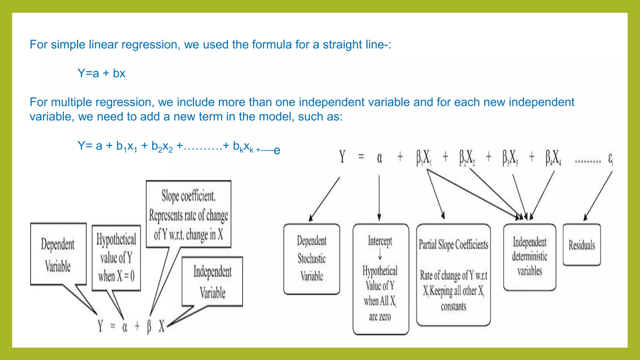
Multiple regression :Regression analysis is used to assess
the relationship between one dependent variable (DV) and
several independent variables (IVs) .
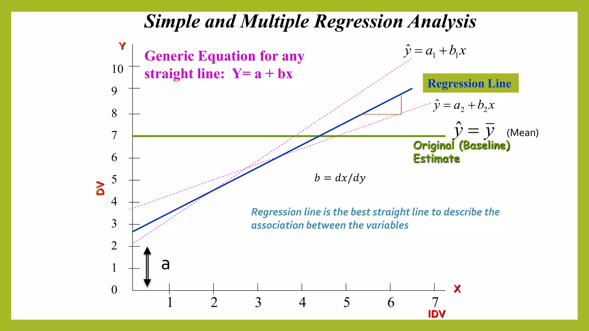
Regression analysis assumes a linear relationship. It focuses
on association, not causation.
Purposes of Regression:
• Prediction
• Explanation-Magnitude ,sign and statistical Significance
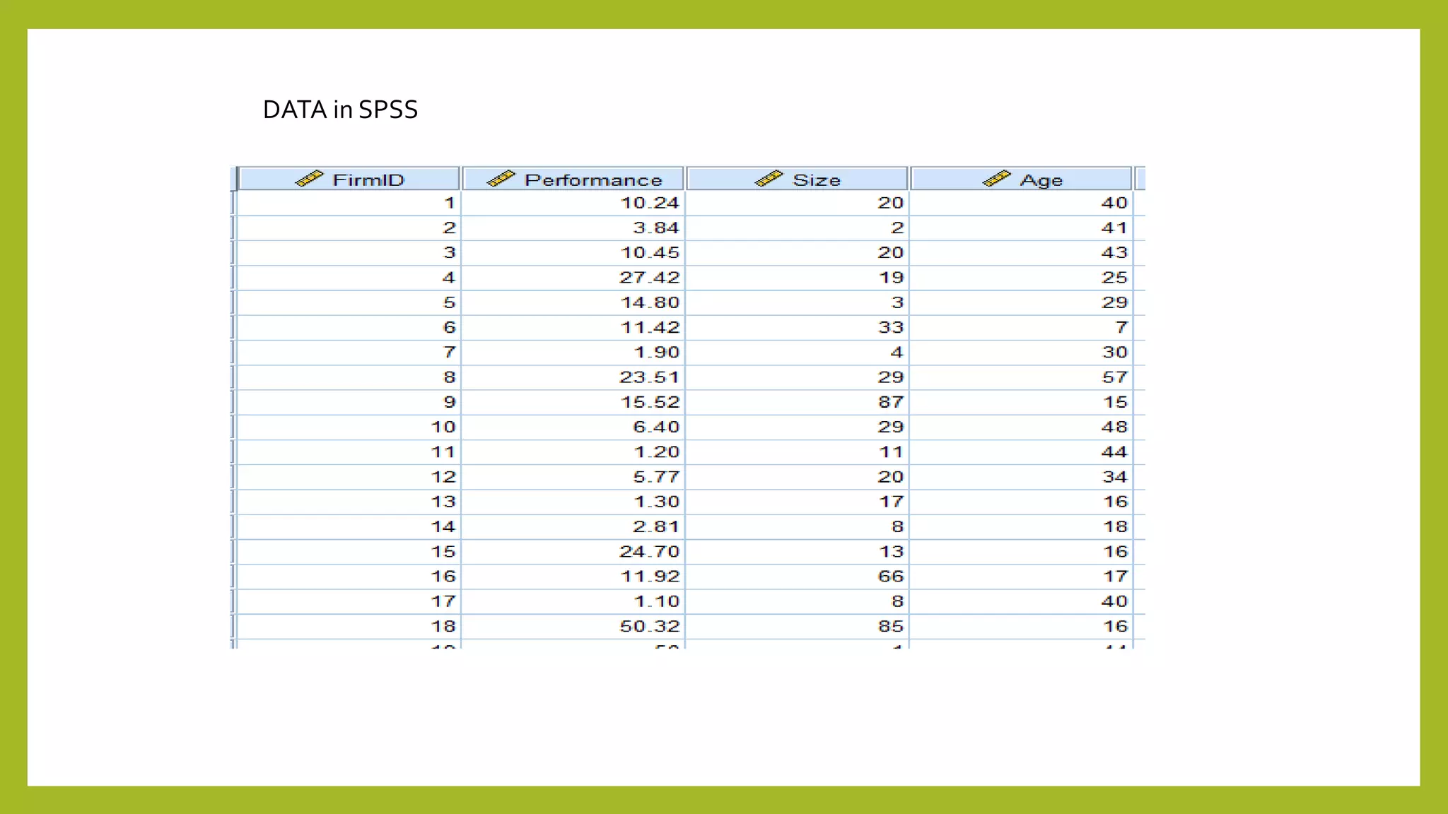
Research Design:
(i) Sample size [5:1]
(ii)Variables- Metric
X1
X2
X3
ŷ

3. For simple linear regression, we used the formula for a straight line-:
Y=a + bx
For multiple regression, we include more than one independent variable and for each new independent
variable, we need to add a new term in the model, such as:
Y= a + b1x1 + b2x2 +……….+ bkxk +-----e

4. Simple and Multiple Regression Analysis
10
9
8
7
6
5
4
3
2
1
0
Y
1 2 3 4 5 6 7
Original (Baseline)
Estimate
X
IDV
Generic Equation for any
straight line: Y= a + bx
x
b
a
y 1
1
ˆ 

x
b
a
y 2
2
ˆ 

Regression Line
y
y 
ˆ
Regression line is the best straight line to describe the
association between the variables
a
𝑏 = 𝑑𝑥/𝑑𝑦
(Mean)

5. Example:
A researcher wants to test some hypotheses regarding the relationship
between size and age of a firm and its performance in a particular industry.
Size was measured by the number of employees working in the firm, age was
the number of years for which the firm has been operating, and performance
was measured by return on equity.
Researcher want to test the following two hypotheses:
H1: Performance of a firm is positively related to its size.
H2: Performance of a firm is positively related to its age.
The null hypotheses in this case would be that performance is not related
to the size or age of the firm.

6. DATA in SPSS

7. SPSS Analysis
Model:
R(Coefficient of Multiple Correlation)
It gives the correlation between observed
and predicted value. >> R is good
Also called Pearson Correlation Coefficient
R2 (Coefficient of Determination)
= Total sum of Square Regression / Total
Sum Of Square
=1179.439/6495.347
=.1815821
Range of R2 between 0 and 1
R2 give model explanatory power
<25% Low ,
>25% Weak Power
>50% Moderate,
>75% Substantial

8. SPSS Analysis
Model:
Adjusted R2 =1 +
𝑛−1
(𝑛 −(𝑘+1)
(1 − R2 )
n= sample size and k=no. of IDV
 Adjusted R2 gives more accurate value
to estimate the R2 for the population.
 IF no. of observation is small : R2 and
Adj R2 have large difference vice versa.
 It means if we add more IDV then value
of R2 will increase and value Adj R2
will also increase but at a certain limit
R2 will increase but adj R2 will be
decrease or constant which shows
adding more IDV’s are not influencing
the outcome and so those IDV’s are
not statistically significant.

9. SPSS Analysis
ANOVA:
P value is less than .05 so it is
statistically fit.
>Regression shows the explained
part and residual shows unexplained
part.
>Initially regression value will be
low and residual value will be high
but by adding more IDV’s regression
value(Explained part ) become high
than residual (Unexplained part) .
>Higher the value of F statistics better
the model fitness
F= ExplainedVariance/Unexplained
variance(ResidualVariance)
=589.720/113.104
=5.214

10. OLS (Ordinary Least Equation) equation
for predicting firm performance (Unstnd.
Beta)
The intercept (a =1.305) is the hypothetical
value of Y when X is zero,this is the point
on Y-axis at which the regression line
passes
Performance = 1.305 + (.185) (Size) +
(0.191) (Age)
We can also construct the regression
equation using Stsnd. Beta if all IVs were
first converted to Z scores.
Z Performance = (0.450) (ZSize) + (0.294) (ZAge)

11. Hypothesis Testing:
The p-value for beta coefficient of Size is 0.003 and
for Age is 0.047. Both these values are significant at
5% significance level. Thus we cannot accept the null
hypothesis and we can claim that the performance of
a firm is positively related to its size and age.

12. Assumptions:
• Independence: the scores of any particular subject are
independent of the scores of all other subjects
• Normality: in the population, the scores on the dependent
variable are normally distributed for each of the possible
combinations of the level of the IDVs variables; each of the
variables is normally distributed
• Linearity: In the population, the relation between the
dependent variable and the independent variable is linear
when all the other independent variables are held constant.
• The error terms should not be correlated with either of the
dependent variable (Y) or the independent variable (X).

13. Collinearity Diagnostics:
Collinearity Statistics gives two values —
Tolerance and VIF (variance inflation
factor). Tolerance is just the inverse of VIF.
A value of VIF higher than three indicates
the presence of multicollinearity.
Both the IDV’s VIF is less than 3 so this
model haven't any multicollinearity.
> Once multicollinearity is detected in the
model, the regression coefficients
are likely to be meaningless. One may
consider removing some IDVs which
are highly correlated to reduce
multicollinearity or club two variables.

14. References:
1. https://www.researchshiksha.com/
2. https://www.youtube.com/watch?v=nD1CiyxVNFo&t=14866s
3. http://math.ucdenver.edu/~ssantori/MATH2830SP13/
4. https://corporatefinanceinstitute.com/resources/knowledge/finance/regression-analysis