Lecture11 xing

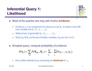
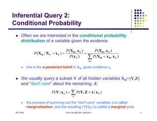
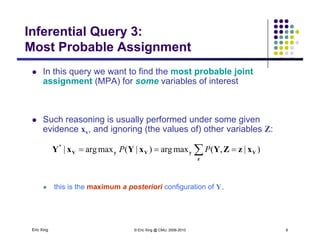
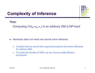
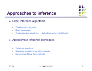
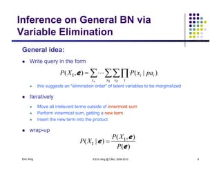
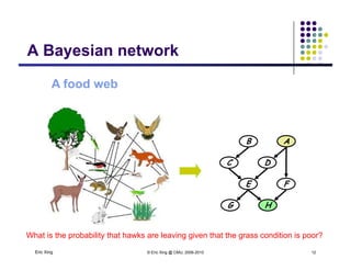
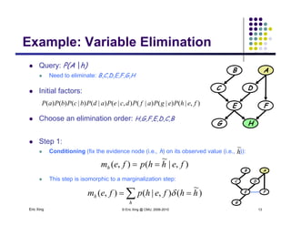
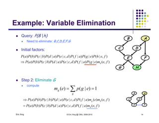
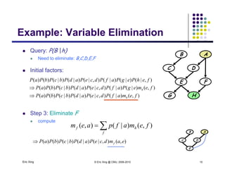
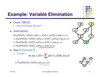
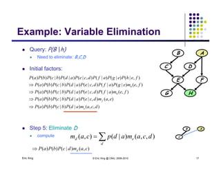
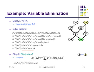
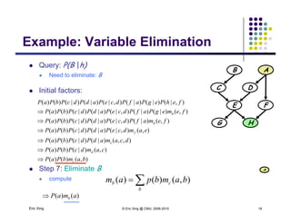
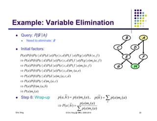
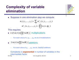
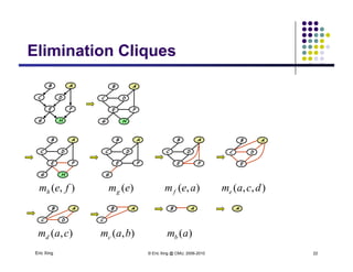
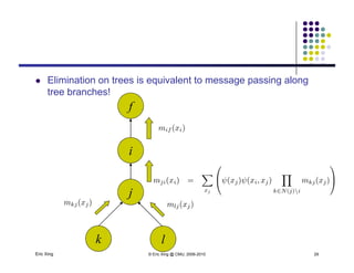
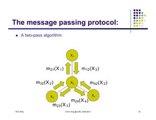
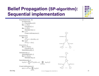
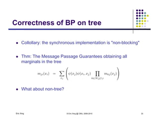
Machine LearningMachine Learninggg
Exact InferenceExact Inference
Eric XingEric Xing
Lecture 11, August 14, 2010
AAA
B A
C
B A
C
B A
C
A
DC
A
DC
B AB A AA
fm
bmcm
dm
Eric Xing © Eric Xing @ CMU, 2006-2010 1
Reading:
E F
H
E F
H
E F
H
E FE FE F
E
G
E
G
E
G
A
DC
E
A
DC
E
A
DC
E
DC DC
hm
gm
em
fm

Inference and LearningInference and Learning
 We now have compact representations of probability
distributions: GM
 A BN M describes a unique probability distribution P
 Typical tasks:
 Task 1: How do we answer queries about P?
 We use inference as a name for the process of computing answers to such
queries
 Task 2: How do we estimate a plausible model M from data D? Task 2: How do we estimate a plausible model M from data D?
i. We use learning as a name for the process of obtaining point estimate of M.
ii. But for Bayesian, they seek p(M |D), which is actually an inference problem.
iii. When not all variables are observable, even computing point estimate of M
need to do inference to impute the missing data.

Inferential Query 1:
LikelihoodLikelihood
 Most of the queries one may ask involve evidenceq y
 Evidence xv is an assignment of values to a set Xv of nodes in the GM
over varialbe set X={X1, X2, …, Xn}
 Without loss of generality Xv={Xk+1, … , Xn},
 Write XH=XXv as the set of hidden variables, XH can be or X
 Simplest query: compute probability of evidence
∑ ∑ )(),,()(
1
1
x x
k
k
,,x,xPPP v
x
vHv xXXx
H
 
 this is often referred to as computing the likelihood of xv

Conditional Probability
 Often we are interested in the conditional probability
Conditional Probability
p y
distribution of a variable given the evidence
VHVH xXxX
xXX
),(),(
)|(
PP
P
 this is the a posteriori belief in XH, given evidence xv
 

Hx
VHH
VH
V
VH
VVH
xxXx
xXX
),()(
)|(
PP
P
this is the a posteriori belief in XH, given evidence xv
 We usually query a subset Y of all hidden variables XH={Y,Z}
and "don't care" about the remaining Z:and don t care about the remaining, Z:
 
z
VV xzZYxY )|,()|( PP
 the process of summing out the "don't care" variables z is called
marginalization, and the resulting P(Y|xv) is called a marginal prob.

Applications of a posteriori Belief
 Prediction: what is the probability of an outcome given the starting
?
Applications of a posteriori Belief
condition
 the query node is a descendent of the evidence
A CB
?
q y
 Diagnosis: what is the probability of disease/fault given symptoms
A CB
?
 the query node an ancestor of the evidence
 Learning under partial observation
A CB
g p
 fill in the unobserved values under an "EM" setting (more later)
 The directionality of information flow between variables is not
y
restricted by the directionality of the edges in a GM
 probabilistic inference can combine evidence form all parts of the network

Most Probable Assignment
 In this query we want to find the most probable joint
Most Probable Assignment
assignment (MPA) for some variables of interest
 Such reasoning is usually performed under some given
evidence xv, and ignoring (the values of) other variables Z:
 
z
VyVyV xzZYxYxY )|,(maxarg)|(maxarg|*
PP
 this is the maximum a posteriori configuration of Y.

Complexity of Inference
Thm:
Complexity of Inference
Thm:
Computing P(XH=xH| xv) in an arbitrary GM is NP-hard
 Hardness does not mean we cannot solve inference
 It implies that we cannot find a general procedure that works efficiently
for arbitrary GMsy
 For particular families of GMs, we can have provably efficient
procedures

Approaches to inferenceApproaches to inference
 Exact inference algorithmsg
 The elimination algorithm
 Belief propagationp p g
 The junction tree algorithms (but will not cover in detail here)
 Approximate inference techniques Approximate inference techniques
 Variational algorithmsVariational algorithms
 Stochastic simulation / sampling methods
 Markov chain Monte Carlo methods

Inference on General BN via
Variable Elimination
General idea:
Variable Elimination
 Write query in the form
  ii paxPXP 1 )|(),( e
 this suggests an "elimination order" of latent variables to be marginalized
 Iteratively
 
nx x x i
ii paxPXP
3 2
1 )|(),( e
 Iteratively
 Move all irrelevant terms outside of innermost sum
 Perform innermost sum, getting a new term
I t th t i t th d t Insert the new term into the product
 wrap-up
),(
)|(
eXP
XP 1
)(
),(
)|(
e
e
P
XP 1
1 

Hidden Markov ModelHidden Markov Model
y2 y3y1 yT...
Conditional probability:
A AA Ax2 x3x1 xT
y2 y3y1 yT...
...

A Bayesian network
A food web
A Bayesian network
A food web
B A
DC
E FE F
G H
What is the probability that hawks are leaving given that the grass condition is poor?

Example: Variable Elimination
 Query: P(A |h)
B A
 Need to eliminate: B,C,D,E,F,G,H
 Initial factors:
B A
DC
 Choose an elimination order: H,G,F,E,D,C,B
E F
G H
),|()|()|(),|()|()|()()( fehPegPafPdcePadPbcPbPaP
 Step 1:
 Conditioning (fix the evidence node (i.e., h) on its observed value (i.e., )):h
~
 This step is isomorphic to a marginalization step:
),|
~
(),( fehhpfemh 
B A
DC
 
h
h hhfehpfem )
~
(),|(),(  E F
G

 Query: P(B |h)
B A
 Need to eliminate: B,C,D,E,F,G
B A
DC
E F
G H
),()|()|(),|()|()|()()(
),|()|()|(),|()|()|()()(
femegPafPdcePadPbcPbPaP
fehPegPafPdcePadPbcPbPaP
h
 Step 2: Eliminate G
t compute
1)|()(  g
g egpem
B A
DC)()()|()|()|()|()()( fememafPdcePadPbcPbPaP h
E F
),()|(),|()|()|()()(
),()()|(),|()|()|()()(
femafPdcePadPbcPbPaP
fememafPdcePadPbcPbPaP
h
hg



 Query: P(B |h)
B A
 Need to eliminate: B,C,D,E,F
B A
DC
E F
G H),()|(),|()|()|()()(
),()|()|(),|()|()|()()(
),|()|()|(),|()|()|()()(
h
h


 Step 3: Eliminate F
t
),()|(),|()|()|()()( ff h
 compute

f
hf femafpaem ),()|(),(
)()|()|()|()()( eamdcePadPbcPbPaP
B A
DC
),(),|()|()|()()( eamdcePadPbcPbPaP f
E

 Query: P(B |h)
B A
 Need to eliminate: B,C,D,E
B A
DC
E F
G H),()|(),|()|()|()()(
),()|()|(),|()|()|()()(
),|()|()|(),|()|()|()()(
h
h


 Step 4: Eliminate E
t
),(),|()|()|()()(
),()|(),|()|()|()()(
eamdcePadPbcPbPaP
ff
f
h

B A
DC
 compute

e
fe eamdcepdcam ),(),|(),,(
)()|()|()()( dcamadPbcPbPaP
B A
DC
E
),,()|()|()()( dcamadPbcPbPaP e

 Query: P(B |h)
B A
 Need to eliminate: B,C,D
B A
DC
E F
G H),()|(),|()|()|()()(
),()|()|(),|()|()|()()(
),|()|()|(),|()|()|()()(
h
h


),,()|()|()()(
),(),|()|()|()()(
dcamadPbcPbPaP
eamdcePadPbcPbPaP
e
f


 Step 5: Eliminate D
 compute
 ed dcamadpcam ),,()|(),(
B A
C
d
ed p ),,()|(),(
),()|()()( camdcPbPaP d

 Query: P(B |h)
B A
 Need to eliminate: B,C
B A
DC
E F
G H),()|(),|()|()|()()(
),()|()|(),|()|()|()()(
),|()|()|(),|()|()|()()(
femafPdcePadPdcPbPaP
femegPafPdcePadPdcPbPaP
fehPegPafPdcePadPdcPbPaP
h
h


),()|()()(
),,()|()|()()(
),(),|()|()|()()(
camdcPbPaP
dcamadPdcPbPaP
eamdcePadPdcPbPaP
d
e
f



 Step 6: Eliminate C
 compute
 dc cambcpbam ),()|(),(
B A
),()|()()( camdcPbPaP d
c
dc p ),()|(),(

 Query: P(B |h)
B A
 Need to eliminate: B
B A
DC
E F
G H),()|(),|()|()|()()(
),()|()|(),|()|()|()()(
),|()|()|(),|()|()|()()(
h
h


),()|()()(
),,()|()|()()(
),(),|()|()|()()(
camdcPbPaP
dcamadPdcPbPaP
eamdcePadPdcPbPaP
d
e
f



 Step 7: Eliminate B
 compute
),()()( bambPaP c
 cb bambpam ),()()(
A
b
cb p ),()()(
)()( amaP b

 Query: P(B |h)
B A
 Need to eliminate: B
B A
DC
E F
G H),()|(),|()|()|()()(
),()|()|(),|()|()|()()(
),|()|()|(),|()|()|()()(
h
h


),()|()()(
),,()|()|()()(
),(),|()|()|()()(
camdcPbPaP
dcamadPdcPbPaP
eamdcePadPdcPbPaP
d
e
f



 Step 8: Wrap-up
)()(
),()()(
amaP
bambPaP
b
c


,)()()
~
,( amaphap b  b amaphp )()()
~
(
Step 8 ap up ,)()(),( pp b


a
b
b
amap
amap
haP
)()(
)()(
)
~
|(
a
b amaphp )()()(

Complexity of variable
elimination
 Suppose in one elimination step we compute
elimination

x
kxkx yyxmyym ),,,('),,( 11 

k
xmyyxm )()(' y
This requires
 multiplications


i
cikx i
xmyyxm
1
1 ),(),,,( y
 CXk )Val()Val( Y p
─ For each value of x, y1, …, yk, we do k multiplications
i
Ci
)()(
 additions
─ For each value of y1, …, yk , we do |Val(X)| additions

i
Ci
X )Val()Val( Y
Complexity is exponential in number of variables in the
intermediate factor

Elimination CliquesElimination Cliques
B AB A
DC
E F
G H
B A
DC
E F
G H
B A
DC
B A
DC
G H
B A
DC
B A
DCD
E F
G H
D
E F
G
DC
E F
DC
E
)( fem )(em )( aem )( dcam
B A
DC
B A
C
B A A
),( femh )(emg ),( aemf ),,( dcame
D
),( camd ),( bamc )(amb

Understanding Variable
EliminationElimination
 A graph elimination algorithm
B A
DC
E F
B A
DC
E F
B A
DC
B A
DC
E F
B A
DC
E F
B A
DC
E
B A
C
B A A
moralization
G H G H G
graph elimination
 Intermediate terms correspond to the cliques resulted from
elimination
 “good” elimination orderings lead to small cliques and hence reduce complexitygood elimination orderings lead to small cliques and hence reduce complexity
(what will happen if we eliminate "e" first in the above graph?)
 finding the optimum ordering is NP-hard, but for many graph optimum or near-
optimum can often be heuristically found
p y
 Applies to undirected GMs

From Elimination to Belief
PropagationPropagation
 Recall that Induced dependency during marginalization isp y g g
captured in elimination cliques
 Summation <-> elimination
 Intermediate term <-> elimination cliqueq
A
B A
C
A
B A A
A
E F
A
DC
A
DC
 Can this lead to an generic
inference algorithm?
E F
H
E
G
E

Tree GMsTree GMs
Undirected tree: a
unique path between
Directed tree: all
nodes except the root
ha e e actl one
Poly tree: can have
multiple parents
any pair of nodes have exactly one
parent

Equivalence of directed and
undirected trees
 Any undirected tree can be converted to a directed tree by choosing a root
undirected trees
node and directing all edges away from it
 A directed tree and the corresponding undirected tree make the same
conditional independence assertionsp
 Parameterizations are essentially the same.
 Undirected tree: Undirected tree:
 Directed tree:
 Equivalence:
 Evidence:?

From elimination to message
passingpassing
 Recall ELIMINATION algorithm:
 Choose an ordering Z in which query node f is the final node
 Place all potentials on an active list
 Eliminate node i by removing all potentials containing i, take sum/product over xi.
Place the resultant factor back on the list Place the resultant factor back on the list
 For a TREE graph:
 Choose query node f as the root of the tree
 View tree as a directed tree with edges pointing towards from f
 Elimination ordering based on depth-first traversal
 Elimination of each node can be considered as message-passing (or Belief Propagation) Elimination of each node can be considered as message passing (or Belief Propagation)
directly along tree branches, rather than on some transformed graphs
 thus, we can use the tree itself as a data-structure to do general inference!!

Message passing for treesMessage passing for trees
Let m (x ) denote the factor resulting from
f
Let mij(xi) denote the factor resulting from
eliminating variables from bellow up to i,
which is a function of xi:
i This is reminiscent of a message sent
from j to i.
j
k l
k l
mij(xi) represents a "belief" of xi from xj!

 Elimination on trees is equivalent to message passing alongq g p g g
tree branches!
f
ii
j
k l

The message passing protocol:The message passing protocol:
 A two-pass algorithm:p g
X1
(X ) (X )
X
m21(X 1)
m32(X 2) m42(X 2)
m12(X 2)
X2
X3
X4
m32(X 2) m42(X 2)
m24(X 4)
3
m23(X 3)

Belief Propagation (SP-algorithm):
Sequential implementationSequential implementation

Belief Propagation (SP-algorithm):
Parallel synchronous implementationParallel synchronous implementation
 For a node of degree d, whenever messages have arrived on any subset of d-1 node,
compute the message for the remaining edge and send!
compute the message for the remaining edge and send!
 A pair of messages have been computed for each edge, one for each direction
 All incoming messages are eventually computed for each node

Correctness of BP on treeCorrectness of BP on tree
 Collollary: the synchronous implementation is "non-blocking"
 Thm: The Message Passage Guarantees obtaining all
marginals in the tree
 What about non-tree?

Inference on general GMInference on general GM
 Now, what if the GM is not a tree-like graph?
 Can we still directly run message
i t l l it d ?message-passing protocol along its edges?
 For non-trees, we do not have the guarantee that message-passingg g p g
will be consistent!
 Then what? Then what?
 Construct a graph data-structure from P that has a tree structure, and run message-passing
on it!
 Junction tree algorithm

Elimination Clique
 Recall that Induced dependency during marginalization is
Elimination Clique
p y g g
captured in elimination cliques
 Summation <-> elimination
 Intermediate term <-> elimination cliqueq
A
B A
C
A
B A A
A
E F
A
DC
A
DC
 Can this lead to an generic
inference algorithm?
E F
H
E
G
E

A Clique TreeA Clique Tree
B A
C
B A A
bmcm
A
C
A
DC
fm
dm
E F
A
DC
E hm
em
E F
H
E
G
E h
gm

e
fg
e
eamemdcep
dcam
),()(),|(
),,(

From Elimination to Message
Passing
 Elimination  message passing on a clique tree
Passing
 Elimination  message passing on a clique tree
B A
DC
E F
B A
DC
E F
B A
DC
B A
DC
E F
B A
DC
E F
B A
DC
E
B A
C
B A A
B A
C
B A A
bmcm
G H G H G

A
E F
A
DC
A
DC
em
fm
dm

e dcam ),,(
E F
H
E
G
DC
E hm
gm

e
fg eamemdcep ),()(),|(
 Messages can be reused

From Elimination to Message
PassingPassing
 Elimination  message passing on a clique tree Elimination  message passing on a clique tree
 Another query ...
B A
C
B A A
cm bm
A
E F
A
DC
A
DC
em
dm
fm
E F
H
E
G
DC
E
gm
hm
 Messages mf and mh are reused, others need to be recomputed

The Shafer Shenoy AlgorithmThe Shafer Shenoy Algorithm
 Shafer-Shenoy algorithmy g
 Message from clique i to clique j :
  S )(
 Clique marginal
 
 
iji
i
SC jk
kiikCji S

)(
 SCp )()( 
 
k
kiikCi SCp i
)()( 

A Sketch of the Junction Tree
AlgorithmAlgorithm
 The algorithmg
 Construction of junction trees --- a special clique tree
 Propagation of probabilities --- a message-passing protocol
 Results in marginal probabilities of all cliques --- solves all
queries in a single run
 A generic exact inference algorithm for any GM A generic exact inference algorithm for any GM
 Complexity: exponential in the size of the maximal clique ---
a good elimination order often leads to small maximal clique,
and hence a good (i.e., thin) JT
 Many well-known algorithms are special cases of JT
 Forward-backward, Kalman filter, Peeling, Sum-Product ...

The Junction tree algorithm for HMMThe Junction tree algorithm for HMM
 A junction tree for the HMM ),( 11 xy ),( 21 yy ),( 32 yy ),( TT yy 1
A AA Ax2 x3x1 xT
y2 y3y1 yT
...
...
y yy yy yy
)( 2y )( 3y )( Ty
)( 1y )( 2y

 Rightward pass ),( 22 xy ),( 33 xy ),( TT xy
),( 1tt yy)( ttt y1 )( 11  ttt y
 )|()()|(
  
ty
tttttttttt yyyyy )()(),()( 11111 
 This is exactly the forward algorithm! ),( 11  tt xy
)( 1 tt
y







t
tt
t
y
tttyytt
y
ttttttt
yayxp
yxpyyyp
)()|(
)|()()|(
, 111
1111
1


y g
 Leftward pass …


 
1
11111
ty
tttttttttt yyyyy )()(),()( 
),( 1tt yy)( ttt y1 )( 11  ttt y
)( 1 ty
 This is exactly the backward algorithm!
1ty



1
11111
ty
ttttttt yxpyyyp )|()()|( 
),( 11  tt xy
)( 1 tt
y

SummarySummary
 The simple Eliminate algorithm captures the key algorithmic
Operation underlying probabilistic inference:
--- That of taking a sum over product of potential functions
 The computational complexity of the Eliminate algorithm can be
reduced to purely graph-theoretic considerations.
 This graph interpretation will also provide hints about how to design
improved inference algorithms
 What can we say about the overall computational complexity of the
algorithm? In particular, how can we control the "size" of the
summands that appear in the sequence of summation operation.

Lecture11 xing

More Related Content

What's hot

Viewers also liked

Similar to Lecture11 xing

More from Tianlu Wang

Recently uploaded

Lecture11 xing