Module
                10
       Reasoning with
          Uncertainty -
Probabilistic reasoning

              Version 2 CSE IIT, Kharagpur
Lesson
                 29
        A Basic Idea of
Inferencing with Bayes
             Networks
              Version 2 CSE IIT, Kharagpur
10.5.5 Inferencing in Bayesian Networks
10.5.5.1 Exact Inference
The basic inference problem in BNs is described as follows:

Given

1. A Bayesian network BN

2. Evidence e - an instantiation of some of the variables in BN (e can be empty)

3. A query variable Q

Compute P(Q|e) - the (marginal) conditional distribution over Q

Given what we do know, compute distribution over what we do not. Four categories of
inferencing tasks are usually encountered.
        1. Diagnostic Inferences (from effects to causes)
             Given that John calls, what is the probability of burglary? i.e. Find P(B|J)
        2. Causal Inferences (from causes to effects)
        Given Burglary, what is the probability that
        John calls, i.e. P(J|B)
        Mary calls, i.e. P(M|B)
        3. Intercausal Inferences (between causes of a common event)
        Given alarm, what is the probability of burglary? i.e. P(B|A)
        Now given Earthquake, what is the probability of burglary? i.e. P(B|A E)
        4. Mixed Inferences (some causes and some effects known)
        Given John calls and no Earth quake, what is the probability of Alarm, i.e.
        P(A|J,~E)

We will demonstrate below the inferencing procedure for BNs. As an example consider
the following linear BN without any apriori evidence.


Consider computing all the marginals (with no evidence). P(A) is given, and


                                                             Version 2 CSE IIT, Kharagpur
We don't need any conditional independence assumption for this.

For example, suppose A, B are binary then we have


Now,


P(B) (the marginal distribution over B) was not given originally. . . but we just computed
it in the last step, so we’re OK (assuming we remembered to store P(B) somewhere).

If C were not independent of A given B, we would have a CPT for P(C|A,B) not
P(C|B).Note that we had to wait for P(B) before P(C) was calculable.

If each node has k values, and the chain has n nodes this algorithm has complexity
O(nk2). Summing over the joint has complexity O(kn).

Complexity can be reduced by more efficient summation by “pushing sums into
products”.


Dynamic programming may also be used for the problem of exact inferencing in the
above Bayes Net. The steps are as follows:

1. We first compute


                                                           Version 2 CSE IIT, Kharagpur
2. f1(B) is a function representable by a table of numbers, one for each possible value of
B.

3. Here,


4. We then use f1(B) to calculate f2(C) by summation over B

This method of solving a problem (ie finding P(D)) by solving subproblems and storing
the results is characteristic of dynamic programming.

The above methodology may be generalized. We eliminated variables starting from the
root, but we dont have to. We might have also done the following computation.


The following points are to be noted about the above algorithm. The algorithm computes
intermediate results which are not individual probabilities, but entire tables such as
f1(C,E). It so happens that f1(C,E) = P(E|C) but we will see examples where the
intermediate tables do not represent probability distributions.

Dealing with Evidence
Dealing with evidence is easy. Suppose {A,B,C,D,E} are all binary and we want
P(C|A = t,E = t). Computing P(C,A = t,E = t) is enough—it’s a table of numbers, one for
each value of C. We need to just renormalise it so that they add up to 1.


                                                            Version 2 CSE IIT, Kharagpur
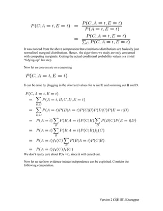
It was noticed from the above computation that conditional distributions are basically just
normalised marginal distributions. Hence, the algorithms we study are only concerned
with computing marginals. Getting the actual conditional probability values is a trivial
“tidying-up” last step.

Now let us concentrate on computing


It can be done by plugging in the observed values for A and E and summing out B and D.


We don’t really care about P(A = t), since it will cancel out.

Now let us see how evidence-induce independence can be exploited. Consider the
following computation.


                                                             Version 2 CSE IIT, Kharagpur
Since,


Clever variable elimination would jump straight to (5). Choosing an optimal order of
variable elimination leads to a large amount of computational sving. However, finding
the optimal order is a hard problem.

10.5.5.1.1 Variable Elimination
For a Bayes net, we can sometimes use the factored representation of the joint probability
distribution to do marginalization efficiently. The key idea is to "push sums in" as far as
possible when summing (marginalizing) out irrelevant terms, e.g., for the water sprinkler
network


Notice that, as we perform the innermost sums, we create new terms, which need to be
summed over in turn e.g.,


where,


Continuing this way,


                                                            Version 2 CSE IIT, Kharagpur
where,


In a nutshell, the variable elimination procedure repeats the following steps.

1. Pick a variable Xi

2. Multiply all expressions involving that variable, resulting in an expression f over a
number of variables (including Xi)

3. Sum out Xi, i.e. compute and store


For the multiplication, we must compute a number for each joint instantiation of all
variables in f, so complexity is exponential in the largest number of variables
participating in one of these multiplicative subexpressions.

If we wish to compute several marginals at the same time, we can use Dynamic
Programming to avoid the redundant computation that would be involved if we used
variable elimination repeatedly.

Exact inferencing in a general Bayes net is a hard problem. However, for networks with
some special topologies efficient solutions inferencing techniques. We discuss one such
technque for a class of networks called Poly-trees.

10.5.5.2 Inferencing in Poly-Trees
A poly-tree is a graph where there is at most one undirected path between any two pair of
nodes. The inferencing problem in poly-trees may be stated as follows.

U: U1 … Um, parents of node X

Y: Y1 … Yn, children of node X

X: Query variable

E: Evidence variables (whose truth values are known)

Objective: compute P(X | E)


                                                             Version 2 CSE IIT, Kharagpur
E+X is the set of causal support for X comprising of the variables above X connected
through its parents, which are known.

E-X is the set of evidential support for X comprising of variables below X connected
through its children.

In order to compute P(X | E) we have

P(X|E) = P(X|EX+,EX-)

           P(EX-|X,EX+)P(X|EX+)
        = -------------------------------
                P(EX-|EX+)

Since X d-separates EX+ from EX- we can simplify the numerator as

P(X|E) = α P(EX-|X)P(X|EX+ )

where 1/α is the constant representing denominator.

Both the terms – P(X|E-X ) and P(E+X|X) can be computed recursively using the
conditional independence relations. If the parents are known, X is conditionally
independent from all other nodes in the Causal support set. Similarly, given the children,
X is independent from all other variables in the evidential support set.

10.5.6 Approximate Inferencing in Bayesian Networks
Many real models of interest, have large number of nodes, which makes exact inference
very slow. Exact inference is NP-hard in the worst case.) We must therefore resort to
approximation techniques. Unfortunately, approximate inference is #P-hard, but we can
nonetheless come up with approximations which often work well in practice. Below is a
list of the major techniques.

Variational methods. The simplest example is the mean-field approximation, which
exploits the law of large numbers to approximate large sums of random variables by their
means. In particular, we essentially decouple all the nodes, and introduce a new
parameter, called a variational parameter, for each node, and iteratively update these
parameters so as to minimize the cross-entropy (KL distance) between the approximate
and true probability distributions. Updating the variational parameters becomes a proxy
for inference. The mean-field approximation produces a lower bound on the likelihood.
More sophisticated methods are possible, which give tighter lower (and upper) bounds.

Sampling (Monte Carlo) methods. The simplest kind is importance sampling, where we
draw random samples x from P(X), the (unconditional) distribution on the hidden
variables, and then weight the samples by their likelihood, P(y|x), where y is the
evidence. A more efficient approach in high dimensions is called Monte Carlo Markov


                                                           Version 2 CSE IIT, Kharagpur
Chain (MCMC), and includes as special cases Gibbs sampling and the Metropolis-
Hasting algorithm.


Bounded cutset conditioning. By instantiating subsets of the variables, we can break
loops in the graph. Unfortunately, when the cutset is large, this is very slow. By
instantiating only a subset of values of the cutset, we can compute lower bounds on the
probabilities of interest. Alternatively, we can sample the cutsets jointly, a technique
known as block Gibbs sampling.

Parametric approximation methods. These express the intermediate summands in a
simpler form, e.g., by approximating them as a product of smaller factors. "Minibuckets"
and the Boyen-Koller algorithm fall into this category.

Questions
1. 1% of women over age forty who are screened, have breast cancer. 80% of women
who really do have breast cancer will have a positive mammography (meaning the test
indicates she has cancer). 9.6% of women who do not actually have breast cancer will
have a positive mammography (meaning that they are incorrectly diagnosed with cancer).
Define two Boolean random variables, M meaning a positive mammography test and ~M
meaning a negative test, and C meaning the woman has breast cancer and ~C means she
does not.

(a) If a woman in this age group gets a positive mammography, what is the probability
that she actually has breast cancer?

(b) True or False: The "Prior" probability, indicating the percentage of women with
breast cancer, is not needed to compute the "Posterior" probability of a woman having
breast cancer given a positive mammography.

(c) Say a woman who gets a positive mammography test, M1, goes back and gets a
second mammography, M2, which also is positive. Use the Naive Bayes assumption to
compute the probability that she has breast cancer given the results from these two tests.

(d) True or False: P(C | M1, M2) can be calculated in general given only P(C) and
P(M1, M2 | C).

2. Let A, B, C, D be Boolean random variables. Given that:

A and B are (absolutely) independent.
C is independent of B given A.
D is independent of C given A and B.
Prob(A=T) = 0.3
Prob(B=T) = 0.6
Prob(C=T|A=T) = 0.8


                                                           Version 2 CSE IIT, Kharagpur
Prob(C=T|A=F) = 0.4
Prob(D=T|A=T,B=T) = 0.7
Prob(D=T|A=T,B=F) = 0.8
Prob(D=T|A=F,B=T) = 0.1
Prob(D=T|A=F,B=F) = 0.2

Compute the following quantities:

1)   Prob(D=T)
2)   Prob(D=F,C=T)
3)   Prob(A=T|C=T)
4)   Prob(A=T|D=F)
5)   Prob(A=T,D=T|B=F).

3. Consider a situation in which we want to reason about the relationship between
smoking and lung cancer. We’ll use 5 Boolean random variables representing "has lung
cancer" (C), "smokes" (S), "has a reduced life expectancy" (RLE), "exposed to second-
hand smoke" (SHS), and "at least one parent smokes" (PS). Intuitively, we know that
whether or not a person has cancer is directly influenced by whether she is exposed to
second-hand smoke and whether she smokes. Both of these things are affected by
whether her parents smoke. Cancer reduces a person’s life expectancy.

i. Draw the network (nodes and arcs only)

ii. How many independent values are required to specify all the conditional probability
tables (CPTs) for your network?

iii. How many independent values are in the full joint probability distribution for this
problem domain?

4. Consider the following Bayesian Network containing 3 Boolean random variables:


(a) Compute the following quantities:

        (i) P(~B, C | A)


                                                             Version 2 CSE IIT, Kharagpur
(ii) P(A | ~B, C)

4.b. Now add on to the network above a fourth node containing Boolean random variable
D, with arcs to it from both B and C.

        (i) Yes or No: Is A conditionally independent of D given B?

        (ii) Yes or No: Is B conditionally independent of C given A?

5. Consider the following probability distribution over 6 variables A,B,C,D,E, and F for
which the factorization as stated below holds. Find and draw a Bayesian network that for
which this factorization is true, but for which no additional factorizations nor any fewer
factorizations are true.


Solution
1.a. Given:
P(C) = 0.01, P(M|C) = 0.8, P(M| ~C) = 0.096.

P(C|M) = [P(M|C)P(C)]/P(M)

= [P(M|C)P(C)]/[P(M|C)P(C) + P(M| C)P( C)]

= (0. 8)(0. 01)/[(0. 8)(0. 01) + (0. 096)(0. 99)]

= (0. 008)/(0. 008 + 0. 09504)

= 0. 0776

So, there is a 7.8% chance.

1.b. False, as seen in the use of Bayes’s Rule in (a).

1.c. P(C|M1, M2) = [P(M1, M2|C)P(C)]/P(M1, M2)
= [P(M1|C)P(M2|C)P(C)]/P(M1, M2)
= (. 8)(. 8)(. 01)/P(M1, M2) = 0. 0064/P(M1, M2)

Now, if we further assume that M1 and M2 are independent, then
P(M1,M2) = P(M1)P(M2) and P(M) = (P(M|C)P(C) + P(M|~C)P(~C)
= (. 8)(. 01) + (. 096)(1-. 01) = 0. 103

Then, P(C|M1,M2) = .0064 / .103 = 0.603 (i.e., 60.3%)


                                                           Version 2 CSE IIT, Kharagpur
More correctly, we don’t assume that M1 and M2 are independent, but only use the
original Naïve Bayes assumption that M1 and M2 are conditionally independent given C.
In this case we need to compute P(M1,M2)

P(M1, M2) = P(M1, M2|C)P(C) + P(M1, Μ2|∼C)P(~C)
= P(M1|C)P(M2|C)P(C) + P(M!|~C)P(M2|~C)P(~C)
= (. 8)(. 8)(. 01) + (. 096)(. 096)(. 99) = 0. 0155

So, P(C|M1,M2) = 0.603 / 0.0155 = 0.4129 (i.e., 41.3%)


1.d. False. Need either P(M1, M2) or P(M1, M2 | ~C).

2. The values of the quantities are given below:

P(D=T) =
P(D=T,A=T,B=T) + P(D=T,A=T,B=F) + P(D=T,A=F,B=T) + P(D=T,A=F,B=F) =
P(D=T|A=T,B=T) P(A=T,B=T) + P(D=T|A=T,B=F) P(A=T,B=F) +
  P(D=T|A=F,B=T) P(A=F,B=T) + P(D=T|A=F,B=F) P(A=F,B=F) =
    (since A and B are independent absolutely)
P(D=T|A=T,B=T) P(A=T) P(B=T) + P(D=T|A=T,B=F) P(A=T) P(B=F) +
  P(D=T|A=F,B=T) P(A=F) P(B=T) + P(D=T|A=F,B=F) P(A=F) P(B=F) =
0.7*0.3*0.6 + 0.8*0.3*0.4 + 0.1*0.7*0.6 + 0.2*0.7*0.4 = 0.32


P(D=F,C=T) =
P(D=F,C=T,A=T,B=T) + P(D=F,C=T,A=T,B=F) + P(D=F,C=T,A=F,B=T) +
P(D=F,C=T,A=F,B=F) =
P(D=F,C=T|A=T,B=T) P(A=T,B=T) + P(D=F,C=T|A=T,B=F) P(A=T,B=F) +
  P(D=F,C=T|A=F,B=T) P(A=F,B=T) + P(D=F,C=T|A=F,B=F) P(A=F,B=F) =
    (since C and D are independent given A and B)
P(D=F|A=T,B=T) P(C=T|A=T,B=T) P(A=T,B=T) + P(D=F|A=T,B=F) P(C=T|A=T,B=F)
P(A=T,B=F) +
  P(D=F|A=F,B=T) P(C=T|A=F,B=T) P(A=F,B=T) +
  P(D=F|A=F,B=F) P(C=T|A=F,B=F) P(A=F,B=F) =
    (since C is independent of B given A and A and B are independent absolutely)
P(D=F|A=T,B=T) P(C=T|A=T) P(A=T) P(B=T) + P(D=F|A=T,B=F) P(C=T|A=T)
P(A=T) P(B=F) +
 P(D=F|A=F,B=T) P(C=T|A=F) P(A=F) P(B=T) + P(D=F|A=F,B=F) P(C=T|A=F)
P(A=F) P(B=F) = 0.3*0.8*0.3*0.6 + 0.2*0.8*0.3*0.4 + 0.9*0.4*0.7*0.6 +
0.8*0.4*0.7*0.4 = 0.3032


P(A=T|C=T) = P(C=T|A=T)P(A=T) / P(C=T).
Now P(C=T) = P(C=T,A=T) + P(C=T,A=F) =
  P(C=T|A=T)P(A=T) + P(C=T|A=F)P(A=F) = 0.8*0.3+ 0.4*0.7 = 0.52


                                                         Version 2 CSE IIT, Kharagpur
So P(C=T|A=T)P(A=T) / P(C=T) = 0.8*0.3/0.52= 0.46.

P(A=T|D=F) = P(D=F|A=T) P(A=T)/P(D=F).
Now P(D=F) = 1-P(D=T) = 0.68 from the first question above.
P(D=F|A=T) = P(D=T,B=T|A=T) + P(D=F,B=F|A=T) =
P(D=F|B=T,A=T) P(B=T|A=T) + P(D=F|B=F,A=T) P(B=F|A=T) =
       (since B is independent of A)
P(D=F|B=T,A=T) P(B=T) + P(D=F|B=F,A=T) P(B=F) = 0.3*0.6 + 0.2*0.4 = 0.26.
So P(A=T|D=F) = P(D=F|A=T) P(A=T)/P(D=F) =
0.26 * 0.3 / 0.68 = 0.115
P(A=T,D=T|B=F) = P(D=T|A=T,B=F) P(A=T|B=F) = (since A and B are independent)
P(D=T|A=T,B=F) P(A=T) = 0.8*0.3 = 0.24.


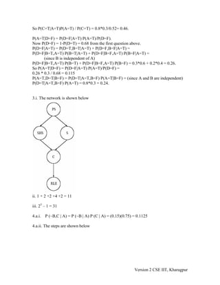
3.i. The network is shown below


ii. 1 + 2 +2 +4 +2 = 11

iii. 25 – 1 = 31

4.a.i.   P (~B,C | A) = P (~B | A) P (C | A) = (0.15)(0.75) = 0.1125

4.a.ii. The steps are shown below


                                                            Version 2 CSE IIT, Kharagpur
4.b.i. No

4.b.ii. Yes

5. The Bayesian network can be obtained by applying chain rule of probability in the
order of factorization mentioned in the question.


                                                          Version 2 CSE IIT, Kharagpur

AI Lesson 29

  • 1.
    Module 10 Reasoning with Uncertainty - Probabilistic reasoning Version 2 CSE IIT, Kharagpur
  • 2.
    Lesson 29 A Basic Idea of Inferencing with Bayes Networks Version 2 CSE IIT, Kharagpur
  • 3.
    10.5.5 Inferencing inBayesian Networks 10.5.5.1 Exact Inference The basic inference problem in BNs is described as follows: Given 1. A Bayesian network BN 2. Evidence e - an instantiation of some of the variables in BN (e can be empty) 3. A query variable Q Compute P(Q|e) - the (marginal) conditional distribution over Q Given what we do know, compute distribution over what we do not. Four categories of inferencing tasks are usually encountered. 1. Diagnostic Inferences (from effects to causes) Given that John calls, what is the probability of burglary? i.e. Find P(B|J) 2. Causal Inferences (from causes to effects) Given Burglary, what is the probability that John calls, i.e. P(J|B) Mary calls, i.e. P(M|B) 3. Intercausal Inferences (between causes of a common event) Given alarm, what is the probability of burglary? i.e. P(B|A) Now given Earthquake, what is the probability of burglary? i.e. P(B|A E) 4. Mixed Inferences (some causes and some effects known) Given John calls and no Earth quake, what is the probability of Alarm, i.e. P(A|J,~E) We will demonstrate below the inferencing procedure for BNs. As an example consider the following linear BN without any apriori evidence. Consider computing all the marginals (with no evidence). P(A) is given, and Version 2 CSE IIT, Kharagpur
  • 4.
    We don't needany conditional independence assumption for this. For example, suppose A, B are binary then we have Now, P(B) (the marginal distribution over B) was not given originally. . . but we just computed it in the last step, so we’re OK (assuming we remembered to store P(B) somewhere). If C were not independent of A given B, we would have a CPT for P(C|A,B) not P(C|B).Note that we had to wait for P(B) before P(C) was calculable. If each node has k values, and the chain has n nodes this algorithm has complexity O(nk2). Summing over the joint has complexity O(kn). Complexity can be reduced by more efficient summation by “pushing sums into products”. Dynamic programming may also be used for the problem of exact inferencing in the above Bayes Net. The steps are as follows: 1. We first compute Version 2 CSE IIT, Kharagpur
  • 5.
    2. f1(B) isa function representable by a table of numbers, one for each possible value of B. 3. Here, 4. We then use f1(B) to calculate f2(C) by summation over B This method of solving a problem (ie finding P(D)) by solving subproblems and storing the results is characteristic of dynamic programming. The above methodology may be generalized. We eliminated variables starting from the root, but we dont have to. We might have also done the following computation. The following points are to be noted about the above algorithm. The algorithm computes intermediate results which are not individual probabilities, but entire tables such as f1(C,E). It so happens that f1(C,E) = P(E|C) but we will see examples where the intermediate tables do not represent probability distributions. Dealing with Evidence Dealing with evidence is easy. Suppose {A,B,C,D,E} are all binary and we want P(C|A = t,E = t). Computing P(C,A = t,E = t) is enough—it’s a table of numbers, one for each value of C. We need to just renormalise it so that they add up to 1. Version 2 CSE IIT, Kharagpur
  • 6.
    It was noticedfrom the above computation that conditional distributions are basically just normalised marginal distributions. Hence, the algorithms we study are only concerned with computing marginals. Getting the actual conditional probability values is a trivial “tidying-up” last step. Now let us concentrate on computing It can be done by plugging in the observed values for A and E and summing out B and D. We don’t really care about P(A = t), since it will cancel out. Now let us see how evidence-induce independence can be exploited. Consider the following computation. Version 2 CSE IIT, Kharagpur
  • 7.
    Since, Clever variable eliminationwould jump straight to (5). Choosing an optimal order of variable elimination leads to a large amount of computational sving. However, finding the optimal order is a hard problem. 10.5.5.1.1 Variable Elimination For a Bayes net, we can sometimes use the factored representation of the joint probability distribution to do marginalization efficiently. The key idea is to "push sums in" as far as possible when summing (marginalizing) out irrelevant terms, e.g., for the water sprinkler network Notice that, as we perform the innermost sums, we create new terms, which need to be summed over in turn e.g., where, Continuing this way, Version 2 CSE IIT, Kharagpur
  • 8.
    where, In a nutshell,the variable elimination procedure repeats the following steps. 1. Pick a variable Xi 2. Multiply all expressions involving that variable, resulting in an expression f over a number of variables (including Xi) 3. Sum out Xi, i.e. compute and store For the multiplication, we must compute a number for each joint instantiation of all variables in f, so complexity is exponential in the largest number of variables participating in one of these multiplicative subexpressions. If we wish to compute several marginals at the same time, we can use Dynamic Programming to avoid the redundant computation that would be involved if we used variable elimination repeatedly. Exact inferencing in a general Bayes net is a hard problem. However, for networks with some special topologies efficient solutions inferencing techniques. We discuss one such technque for a class of networks called Poly-trees. 10.5.5.2 Inferencing in Poly-Trees A poly-tree is a graph where there is at most one undirected path between any two pair of nodes. The inferencing problem in poly-trees may be stated as follows. U: U1 … Um, parents of node X Y: Y1 … Yn, children of node X X: Query variable E: Evidence variables (whose truth values are known) Objective: compute P(X | E) Version 2 CSE IIT, Kharagpur
  • 9.
    E+X is theset of causal support for X comprising of the variables above X connected through its parents, which are known. E-X is the set of evidential support for X comprising of variables below X connected through its children. In order to compute P(X | E) we have P(X|E) = P(X|EX+,EX-) P(EX-|X,EX+)P(X|EX+) = ------------------------------- P(EX-|EX+) Since X d-separates EX+ from EX- we can simplify the numerator as P(X|E) = α P(EX-|X)P(X|EX+ ) where 1/α is the constant representing denominator. Both the terms – P(X|E-X ) and P(E+X|X) can be computed recursively using the conditional independence relations. If the parents are known, X is conditionally independent from all other nodes in the Causal support set. Similarly, given the children, X is independent from all other variables in the evidential support set. 10.5.6 Approximate Inferencing in Bayesian Networks Many real models of interest, have large number of nodes, which makes exact inference very slow. Exact inference is NP-hard in the worst case.) We must therefore resort to approximation techniques. Unfortunately, approximate inference is #P-hard, but we can nonetheless come up with approximations which often work well in practice. Below is a list of the major techniques. Variational methods. The simplest example is the mean-field approximation, which exploits the law of large numbers to approximate large sums of random variables by their means. In particular, we essentially decouple all the nodes, and introduce a new parameter, called a variational parameter, for each node, and iteratively update these parameters so as to minimize the cross-entropy (KL distance) between the approximate and true probability distributions. Updating the variational parameters becomes a proxy for inference. The mean-field approximation produces a lower bound on the likelihood. More sophisticated methods are possible, which give tighter lower (and upper) bounds. Sampling (Monte Carlo) methods. The simplest kind is importance sampling, where we draw random samples x from P(X), the (unconditional) distribution on the hidden variables, and then weight the samples by their likelihood, P(y|x), where y is the evidence. A more efficient approach in high dimensions is called Monte Carlo Markov Version 2 CSE IIT, Kharagpur
  • 10.
    Chain (MCMC), andincludes as special cases Gibbs sampling and the Metropolis- Hasting algorithm. Bounded cutset conditioning. By instantiating subsets of the variables, we can break loops in the graph. Unfortunately, when the cutset is large, this is very slow. By instantiating only a subset of values of the cutset, we can compute lower bounds on the probabilities of interest. Alternatively, we can sample the cutsets jointly, a technique known as block Gibbs sampling. Parametric approximation methods. These express the intermediate summands in a simpler form, e.g., by approximating them as a product of smaller factors. "Minibuckets" and the Boyen-Koller algorithm fall into this category. Questions 1. 1% of women over age forty who are screened, have breast cancer. 80% of women who really do have breast cancer will have a positive mammography (meaning the test indicates she has cancer). 9.6% of women who do not actually have breast cancer will have a positive mammography (meaning that they are incorrectly diagnosed with cancer). Define two Boolean random variables, M meaning a positive mammography test and ~M meaning a negative test, and C meaning the woman has breast cancer and ~C means she does not. (a) If a woman in this age group gets a positive mammography, what is the probability that she actually has breast cancer? (b) True or False: The "Prior" probability, indicating the percentage of women with breast cancer, is not needed to compute the "Posterior" probability of a woman having breast cancer given a positive mammography. (c) Say a woman who gets a positive mammography test, M1, goes back and gets a second mammography, M2, which also is positive. Use the Naive Bayes assumption to compute the probability that she has breast cancer given the results from these two tests. (d) True or False: P(C | M1, M2) can be calculated in general given only P(C) and P(M1, M2 | C). 2. Let A, B, C, D be Boolean random variables. Given that: A and B are (absolutely) independent. C is independent of B given A. D is independent of C given A and B. Prob(A=T) = 0.3 Prob(B=T) = 0.6 Prob(C=T|A=T) = 0.8 Version 2 CSE IIT, Kharagpur
  • 11.
    Prob(C=T|A=F) = 0.4 Prob(D=T|A=T,B=T)= 0.7 Prob(D=T|A=T,B=F) = 0.8 Prob(D=T|A=F,B=T) = 0.1 Prob(D=T|A=F,B=F) = 0.2 Compute the following quantities: 1) Prob(D=T) 2) Prob(D=F,C=T) 3) Prob(A=T|C=T) 4) Prob(A=T|D=F) 5) Prob(A=T,D=T|B=F). 3. Consider a situation in which we want to reason about the relationship between smoking and lung cancer. We’ll use 5 Boolean random variables representing "has lung cancer" (C), "smokes" (S), "has a reduced life expectancy" (RLE), "exposed to second- hand smoke" (SHS), and "at least one parent smokes" (PS). Intuitively, we know that whether or not a person has cancer is directly influenced by whether she is exposed to second-hand smoke and whether she smokes. Both of these things are affected by whether her parents smoke. Cancer reduces a person’s life expectancy. i. Draw the network (nodes and arcs only) ii. How many independent values are required to specify all the conditional probability tables (CPTs) for your network? iii. How many independent values are in the full joint probability distribution for this problem domain? 4. Consider the following Bayesian Network containing 3 Boolean random variables: (a) Compute the following quantities: (i) P(~B, C | A) Version 2 CSE IIT, Kharagpur
  • 12.
    (ii) P(A |~B, C) 4.b. Now add on to the network above a fourth node containing Boolean random variable D, with arcs to it from both B and C. (i) Yes or No: Is A conditionally independent of D given B? (ii) Yes or No: Is B conditionally independent of C given A? 5. Consider the following probability distribution over 6 variables A,B,C,D,E, and F for which the factorization as stated below holds. Find and draw a Bayesian network that for which this factorization is true, but for which no additional factorizations nor any fewer factorizations are true. Solution 1.a. Given: P(C) = 0.01, P(M|C) = 0.8, P(M| ~C) = 0.096. P(C|M) = [P(M|C)P(C)]/P(M) = [P(M|C)P(C)]/[P(M|C)P(C) + P(M| C)P( C)] = (0. 8)(0. 01)/[(0. 8)(0. 01) + (0. 096)(0. 99)] = (0. 008)/(0. 008 + 0. 09504) = 0. 0776 So, there is a 7.8% chance. 1.b. False, as seen in the use of Bayes’s Rule in (a). 1.c. P(C|M1, M2) = [P(M1, M2|C)P(C)]/P(M1, M2) = [P(M1|C)P(M2|C)P(C)]/P(M1, M2) = (. 8)(. 8)(. 01)/P(M1, M2) = 0. 0064/P(M1, M2) Now, if we further assume that M1 and M2 are independent, then P(M1,M2) = P(M1)P(M2) and P(M) = (P(M|C)P(C) + P(M|~C)P(~C) = (. 8)(. 01) + (. 096)(1-. 01) = 0. 103 Then, P(C|M1,M2) = .0064 / .103 = 0.603 (i.e., 60.3%) Version 2 CSE IIT, Kharagpur
  • 13.
    More correctly, wedon’t assume that M1 and M2 are independent, but only use the original Naïve Bayes assumption that M1 and M2 are conditionally independent given C. In this case we need to compute P(M1,M2) P(M1, M2) = P(M1, M2|C)P(C) + P(M1, Μ2|∼C)P(~C) = P(M1|C)P(M2|C)P(C) + P(M!|~C)P(M2|~C)P(~C) = (. 8)(. 8)(. 01) + (. 096)(. 096)(. 99) = 0. 0155 So, P(C|M1,M2) = 0.603 / 0.0155 = 0.4129 (i.e., 41.3%) 1.d. False. Need either P(M1, M2) or P(M1, M2 | ~C). 2. The values of the quantities are given below: P(D=T) = P(D=T,A=T,B=T) + P(D=T,A=T,B=F) + P(D=T,A=F,B=T) + P(D=T,A=F,B=F) = P(D=T|A=T,B=T) P(A=T,B=T) + P(D=T|A=T,B=F) P(A=T,B=F) + P(D=T|A=F,B=T) P(A=F,B=T) + P(D=T|A=F,B=F) P(A=F,B=F) = (since A and B are independent absolutely) P(D=T|A=T,B=T) P(A=T) P(B=T) + P(D=T|A=T,B=F) P(A=T) P(B=F) + P(D=T|A=F,B=T) P(A=F) P(B=T) + P(D=T|A=F,B=F) P(A=F) P(B=F) = 0.7*0.3*0.6 + 0.8*0.3*0.4 + 0.1*0.7*0.6 + 0.2*0.7*0.4 = 0.32 P(D=F,C=T) = P(D=F,C=T,A=T,B=T) + P(D=F,C=T,A=T,B=F) + P(D=F,C=T,A=F,B=T) + P(D=F,C=T,A=F,B=F) = P(D=F,C=T|A=T,B=T) P(A=T,B=T) + P(D=F,C=T|A=T,B=F) P(A=T,B=F) + P(D=F,C=T|A=F,B=T) P(A=F,B=T) + P(D=F,C=T|A=F,B=F) P(A=F,B=F) = (since C and D are independent given A and B) P(D=F|A=T,B=T) P(C=T|A=T,B=T) P(A=T,B=T) + P(D=F|A=T,B=F) P(C=T|A=T,B=F) P(A=T,B=F) + P(D=F|A=F,B=T) P(C=T|A=F,B=T) P(A=F,B=T) + P(D=F|A=F,B=F) P(C=T|A=F,B=F) P(A=F,B=F) = (since C is independent of B given A and A and B are independent absolutely) P(D=F|A=T,B=T) P(C=T|A=T) P(A=T) P(B=T) + P(D=F|A=T,B=F) P(C=T|A=T) P(A=T) P(B=F) + P(D=F|A=F,B=T) P(C=T|A=F) P(A=F) P(B=T) + P(D=F|A=F,B=F) P(C=T|A=F) P(A=F) P(B=F) = 0.3*0.8*0.3*0.6 + 0.2*0.8*0.3*0.4 + 0.9*0.4*0.7*0.6 + 0.8*0.4*0.7*0.4 = 0.3032 P(A=T|C=T) = P(C=T|A=T)P(A=T) / P(C=T). Now P(C=T) = P(C=T,A=T) + P(C=T,A=F) = P(C=T|A=T)P(A=T) + P(C=T|A=F)P(A=F) = 0.8*0.3+ 0.4*0.7 = 0.52 Version 2 CSE IIT, Kharagpur
  • 14.
    So P(C=T|A=T)P(A=T) /P(C=T) = 0.8*0.3/0.52= 0.46. P(A=T|D=F) = P(D=F|A=T) P(A=T)/P(D=F). Now P(D=F) = 1-P(D=T) = 0.68 from the first question above. P(D=F|A=T) = P(D=T,B=T|A=T) + P(D=F,B=F|A=T) = P(D=F|B=T,A=T) P(B=T|A=T) + P(D=F|B=F,A=T) P(B=F|A=T) = (since B is independent of A) P(D=F|B=T,A=T) P(B=T) + P(D=F|B=F,A=T) P(B=F) = 0.3*0.6 + 0.2*0.4 = 0.26. So P(A=T|D=F) = P(D=F|A=T) P(A=T)/P(D=F) = 0.26 * 0.3 / 0.68 = 0.115 P(A=T,D=T|B=F) = P(D=T|A=T,B=F) P(A=T|B=F) = (since A and B are independent) P(D=T|A=T,B=F) P(A=T) = 0.8*0.3 = 0.24. 3.i. The network is shown below ii. 1 + 2 +2 +4 +2 = 11 iii. 25 – 1 = 31 4.a.i. P (~B,C | A) = P (~B | A) P (C | A) = (0.15)(0.75) = 0.1125 4.a.ii. The steps are shown below Version 2 CSE IIT, Kharagpur
  • 15.
    4.b.i. No 4.b.ii. Yes 5.The Bayesian network can be obtained by applying chain rule of probability in the order of factorization mentioned in the question. Version 2 CSE IIT, Kharagpur