Download as PDF, PPTX


![]
)
|
,
(
)
|
,
(
[log
]
)
|
,
(
)
|
,
(
[
log
)
|
,
(
)
|
,
(
)
,
|
(
log
)
|
,
(
)
|
,
(
)
|
'
,
(
)
|
,
(
log
)
|
,
(
)
|
,
(
)
|
'
,
(
)
|
,
(
log
)
|
'
,
(
)
|
,
(
log
)
|
,
(
)
|
,
(
log
)
|
,
(
log
)
|
,
(
log
)
|
(
log
)
|
(
log
)
(
)
(
1
)
,
|
(
1
)
,
|
(
1
'
1
'
1
'
1
1
1
1
t
i
i
n
i
x
y
P
t
i
i
n
i
x
y
P
t
i
i
t
n
i y
i
t
i
i
y
t
y
i
t
i
n
i
t
i
t
i
y
t
y
i
i
n
i
y
t
y
i
i
n
i
t
y
i
y
i
n
i
t
y
i
n
i
y
i
n
i
t
t
y
x
P
y
x
P
E
y
x
P
y
x
P
E
y
x
P
y
x
P
x
y
P
y
x
P
y
x
P
y
x
P
y
x
P
y
x
P
y
x
P
y
x
P
y
x
P
y
x
P
y
x
P
y
x
P
y
x
P
y
x
P
y
x
P
X
P
X
P
l
l
t
i
t
i
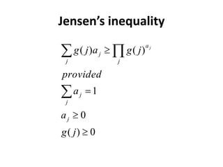
Jensen’s inequality](https://image.slidesharecdn.com/mlmapreduce-240622083506-576a697f/85/Machine-Learning-With-MapReduce-K-Means-MLE-17-320.jpg)
![Jensen’s inequality
])
(
[
(
)]
(
(
[
, x
g
E
f
x
g
f
E
then
convex
is
f
if
)])
(
[
log(
)]
(
[log( x
p
E
x
p
E
])
(
[
(
)]
(
(
[
, x
g
E
f
x
g
f
E
then
concave
is
f
if
log is a concave function](https://image.slidesharecdn.com/mlmapreduce-240622083506-576a697f/85/Machine-Learning-With-MapReduce-K-Means-MLE-18-320.jpg)
![Maximizing the lower bound
)]
|
,
(
[log
max
arg
)
|
,
(
log
)
,
|
(
max
arg
)
|
,
(
)
|
,
(
log
)
,
|
(
max
arg
]
)
|
,
(
)
|
,
(
[log
max
arg
1
)
,
|
(
1
1
1
)
,
|
(
)
1
(
y
x
P
E
y
x
P
x
y
P
y
x
P
y
x
P
x
y
P
y
x
p
y
x
p
E
i
n
i
x
y
P
i
t
i
n
i y
t
i
i
t
i
n
i y
t
i
i
n
i
x
y
P
t
t
i
t
i
The Q function](https://image.slidesharecdn.com/mlmapreduce-240622083506-576a697f/85/Machine-Learning-With-MapReduce-K-Means-MLE-19-320.jpg)
![The Q-function
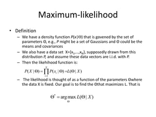
• Define the Q-function (a function of θ):
– Y is a random vector.
– X=(x1, x2, …, xn) is a constant (vector).
– Θt is the current parameter estimate and is a constant (vector).
– Θ is the normal variable (vector) that we wish to adjust.
• The Q-function is the expected value of the complete data log-likelihood
P(X,Y|θ) with respect to Y given X and θt.
)
|
,
(
log
)
,
|
(
)]
|
,
(
[log
)
|
,
(
log
)
,
|
(
)]
|
,
(
[log
]
,
|
)
|
,
(
[log
)
,
(
1
1
)
,
|
(
)
,
|
(
y
x
P
x
y
P
y
x
P
E
Y
X
P
X
Y
P
Y
X
P
E
X
Y
X
P
E
Q
i
t
n
i y
i
n
i
i
x
y
P
Y
t
X
Y
P
t
t
t
i
t
](https://image.slidesharecdn.com/mlmapreduce-240622083506-576a697f/85/Machine-Learning-With-MapReduce-K-Means-MLE-20-320.jpg)

![Idea #3: find θt+1 that maximizes a tight
lower bound of )
(
)
( t
l
l
a tight lower bound
]
)
|
,
(
)
|
,
(
[log
)
(
)
(
1
)
,
|
( t
i
i
n
i
x
y
P
t
y
x
P
y
x
P
E
l
l t
i
](https://image.slidesharecdn.com/mlmapreduce-240622083506-576a697f/85/Machine-Learning-With-MapReduce-K-Means-MLE-27-320.jpg)
![Idea #4: find θt+1 that maximizes
the Q function
)]
|
,
(
[log
max
arg
]
)
|
,
(
)
|
,
(
[log
max
arg
1
)
,
|
(
1
)
,
|
(
)
1
(
y
x
P
E
y
x
p
y
x
p
E
i
n
i
x
y
P
t
i
i
n
i
x
y
P
t
t
i
t
i
Lower bound of )
(
)
( t
l
l
The Q function](https://image.slidesharecdn.com/mlmapreduce-240622083506-576a697f/85/Machine-Learning-With-MapReduce-K-Means-MLE-28-320.jpg)
![
D
d W
w Z
z
z
d
P
z
w
P
z
P
w
d
n
z
w
d
L )
|
(
)
|
(
)
(
log
)
,
(
max
)
,
,
|
(
max
Estimation-using EM
difficult!!!
Idea: start with a guess t, compute an easily computed lower-bound B(; t)
to the function log P(|U) and maximize the bound instead
By Jensen’s inequality:
)
,
|
(
]
)
,
|
(
)
|
(
)
|
(
)
(
[
)
,
|
(
)
,
|
(
)
|
(
)
|
(
)
(
d
w
z
P
Z
z j d
w
z
P
z
d
P
z
w
P
z
P
d
w
z
P
d
w
z
P
z
d
P
z
w
P
z
P
D
d W
w z
d
w
z
P
z
D
d W
w
t
d
w
z
P
d
w
z
P
z
d
P
z
w
P
z
P
w
d
n
d
w
z
P
z
d
P
z
w
P
z
P
w
d
n
B
)
,
|
(
)]
,
|
(
log
)
|
(
)
|
(
)
(
[log
)
,
(
max
]
)
,
|
(
)
|
(
)
|
(
)
(
[
log
)
,
(
max
)
,
(
max
)
,
|
(](https://image.slidesharecdn.com/mlmapreduce-240622083506-576a697f/85/Machine-Learning-With-MapReduce-K-Means-MLE-36-320.jpg)
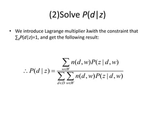
![(1)Solve P(w|z)
• We introduce Lagrange multiplier λwith the constraint that
∑wP(w|z)=1, and solve the following equation:
( , ) [log ( ) ( | ) ( | ) log ( | , )] ( | , ) ( ( | ) 1) 0
( | )
( , ) ( | , )
0,
( | )
( , ) ( | , )
( | ) ,
( | ) 1,
( , ) ( | , ),
( , )
( | )
d D w W z w
d D
d D
w
w W d D
n d w P z P w z P d z P z w d P z w d P w z
P w z
n d w P z d w
P w z
n d w P z d w
P w z
P w z
n d w P z d w
n d w P
P w z
( | , )
( , ) ( | , )
d D
w W d D
z d w
n d w P z d w
](https://image.slidesharecdn.com/mlmapreduce-240622083506-576a697f/85/Machine-Learning-With-MapReduce-K-Means-MLE-37-320.jpg)
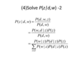
![(3)Solve P(z)
• We introduce Lagrange multiplier λwith the constraint that
∑zP(z)=1, and solve the following equation:
( , ) [log ( ) ( | ) ( | ) log ( | , )] ( | , ) ( ( ) 1) 0
( )
( , ) ( | , )
0,
( )
( , ) ( | , )
( ) ,
( ) 1,
( , ) ( | , ) ( , ),
d D w W z z
d D w W
d D w W
z
d D w W z d D w W
n d w P z P w z P d z P z w d P z w d P z
P z
n d w P z d w
P z
n d w P z d w
P z
P z
n d w P z d w n d w
( , ) ( | , )
( )
( , )
d D w W
w W d D
n d w P z d w
P z
n d w
](https://image.slidesharecdn.com/mlmapreduce-240622083506-576a697f/85/Machine-Learning-With-MapReduce-K-Means-MLE-39-320.jpg)
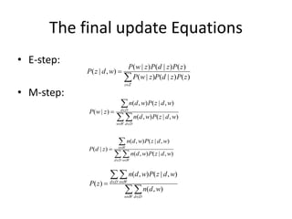
![(1)Solve P(z|d,w)
• We introduce Lagrange multiplier λwith the constraint that
∑zP(z|d,w)=1, and solve the following equation:
,
,
,
( , ) [log ( ) ( | ) ( | ) log ( | , )] ( | , ) ( ( | , ) 1) 0
( | , )
( , )[log ( ) ( | ) ( | ) log ( | , ) 1] 0,
log ( | , ) log ( ) ( | ) ( | ) 1 0,
( |
d w
d D w W z d D w W z
d w
d w
n d w P z P w z P d z P z d w P z d w P z d w
P z d w
n d w P z P w z P d z P z d w
P z d w P z P w z P d z
P z d
,
,
,
1
1
,
1
1 (1 log ( ) ( | ) ( | ))
, ) ( ) ( | ) ( | )
( | , ) 1,
( ) ( | ) ( | ) 1
1 log ( ) ( | ) ( | )
( ) ( | ) ( | )
( | )
( ) ( | ) ( | )
( ) ( | ) ( | )
( ) ( |
d w
d w
d w
z
z
z
d w
z
P z P w z P d z
w P z P w z P d z e
P z d w
P z P w z P d z e
P z P w z P d z
P z P w z P d z
P w z
e
P z P w z P d z
e
P z P w z P d z
P z P w z
) ( | )
z
P d z
](https://image.slidesharecdn.com/mlmapreduce-240622083506-576a697f/85/Machine-Learning-With-MapReduce-K-Means-MLE-40-320.jpg)
![Coding Design
• Variables:
• double[][] p_dz_n // p(d|z), |D|*|Z|
• double[][] p_wz_n // p(w|z), |W|*|Z|
• double[] p_z_n // p(z), |Z|
• Running Processing:
1. Read dataset from file
ArrayList<DocWordPair> doc; // all the docs
DocWordPair – (word_id, word_frequency_in_doc)
2. Parameter Initialization
Assign each elements of p_dz_n, p_wz_n and p_z_n with a random double value, satisfying
∑d p_dz_n=1, ∑d p_wz_n =1, and ∑d p_z_n =1
3. Estimation (Iterative processing)
1. Update p_dz_n, p_wz_n and p_z_n
2. Calculate Log-likelihood function to see where ( |Log-likelihood – old_Log-likelihood|
< threshold)
4. Output p_dz_n, p_wz_n and p_z_n](https://image.slidesharecdn.com/mlmapreduce-240622083506-576a697f/85/Machine-Learning-With-MapReduce-K-Means-MLE-43-320.jpg)
![Coding Design
• Update p_dz_n
For each doc d{
For each word w included in d {
denominator = 0;
nominator = new double[Z];
For each topic z {
nominator[z] = p_dz_n[d][z]* p_wz_n[w][z]* p_z_n[z]
denominator +=nominator[z];
} // end for each topic z
For each topic z {
P_z_condition_d_w = nominator[j]/denominator;
nominator_p_dz_n[d][z] += tfwd*P_z_condition_d_w;
denominator_p_dz_n[z] += tfwd*P_z_condition_d_w;
} // end for each topic z
}// end for each word w included in d
}// end for each doc d
For each doc d {
For each topic z {
p_dz_n_new[d][z] = nominator_p_dz_n[d][z]/ denominator_p_dz_n[z];
} // end for each topic z
}// end for each doc d](https://image.slidesharecdn.com/mlmapreduce-240622083506-576a697f/85/Machine-Learning-With-MapReduce-K-Means-MLE-44-320.jpg)
![Coding Design
• Update p_wz_n
For each doc d{
For each word w included in d {
denominator = 0;
nominator = new double[Z];
For each topic z {
nominator[z] = p_dz_n[d][z]* p_wz_n[w][z]* p_z_n[z]
denominator +=nominator[z];
} // end for each topic z
For each topic z {
P_z_condition_d_w = nominator[j]/denominator;
nominator_p_wz_n[w][z] += tfwd*P_z_condition_d_w;
denominator_p_wz_n[z] += tfwd*P_z_condition_d_w;
} // end for each topic z
}// end for each word w included in d
}// end for each doc d
For each w {
For each topic z {
p_wz_n_new[w][z] = nominator_p_wz_n[w][z]/ denominator_p_wz_n[z];
} // end for each topic z
}// end for each doc d](https://image.slidesharecdn.com/mlmapreduce-240622083506-576a697f/85/Machine-Learning-With-MapReduce-K-Means-MLE-45-320.jpg)
![Coding Design
• Update p_z_n
For each doc d{
For each word w included in d {
denominator = 0;
nominator = new double[Z];
For each topic z {
nominator[z] = p_dz_n[d][z]* p_wz_n[w][z]* p_z_n[z]
denominator +=nominator[z];
} // end for each topic z
For each topic z {
P_z_condition_d_w = nominator[j]/denominator;
nominator_p_z_n[z] += tfwd*P_z_condition_d_w;
} // end for each topic z
denominator_p_z_n[z] += tfwd;
}// end for each word w included in d
}// end for each doc d
For each topic z{
p_dz_n_new[d][j] = nominator_p_z_n[z]/ denominator_p_z_n;
} // end for each topic z](https://image.slidesharecdn.com/mlmapreduce-240622083506-576a697f/85/Machine-Learning-With-MapReduce-K-Means-MLE-46-320.jpg)


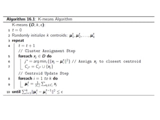
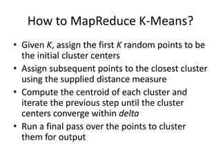
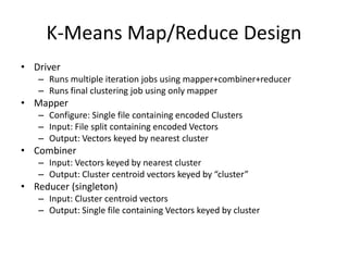
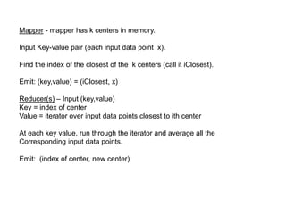
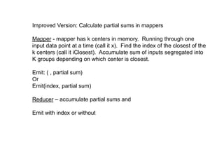
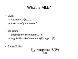
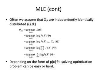
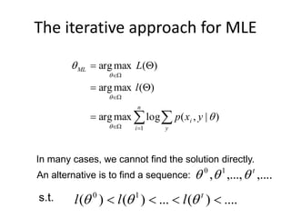
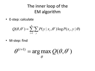
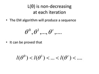
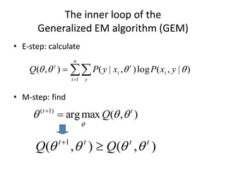
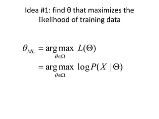
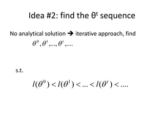
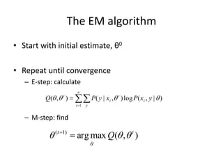
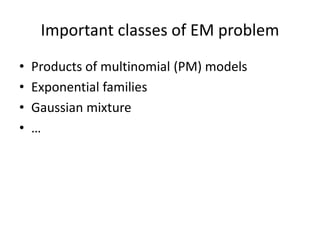
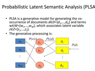
The document outlines the application of MapReduce to k-means clustering, detailing the process of assigning initial cluster centers, iteratively updating clusters, and finalizing the output. It discusses the Expectation-Maximization (EM) algorithm for parameter estimation in probabilistic models, highlighting the steps involved in maximizing the log-likelihood through iterative calculations. Additionally, the document introduces concepts related to probabilistic latent semantic analysis (PLSA), emphasizing the generative process for documents and terms using latent variables.


![[DSC Europe 25] Mikhail Rozhkov - AI Product Canvas: From Business Goals to T...](https://cdn.slidesharecdn.com/ss_thumbnails/d53doddtpgfqivmzqel6-mikhail-rozhkov-ai-product-canvas-v1-260121115910-9dd517a7-thumbnail.jpg?width=640&height=640&fit=bounds)

![[DSC Europe 25] Andrzej Kowalczyk - AI - how to start small and grow in the f...](https://cdn.slidesharecdn.com/ss_thumbnails/oy1zmo94qv6vpcqjvno2-andrzej-kowalczyk-ai-how-to-start-small-and-grow-in-the-future-1-260119121559-cf093b23-thumbnail.jpg?width=640&height=640&fit=bounds)


![[DSC Europe 25] Dubravko Culibrk - Deep Learning for Mammography.pptx](https://cdn.slidesharecdn.com/ss_thumbnails/yiscimuktacgqoiu4dkp-deep-learning-for-mammography-260119121559-aad59182-thumbnail.jpg?width=640&height=640&fit=bounds)


![[DSC Europe 25] Tamas Srancsik - How To Teach Your AI Football? An Argument f...](https://cdn.slidesharecdn.com/ss_thumbnails/bcjh1m9xtbosv20ucftb-tamas-srancsik-how-to-teach-your-ai-football-260121115910-08b53e9e-thumbnail.jpg?width=640&height=640&fit=bounds)
![[DSC Europe 25] Bojan Djuricic - Predictive Design Process.pdf](https://cdn.slidesharecdn.com/ss_thumbnails/5awdrbedqdek3gqu2ezy-4-the-predictive-design-bojan-djuricic-260120105856-6c399e9b-thumbnail.jpg?width=640&height=640&fit=bounds)

![[DSC Europe 25] Marcos Heidemann - Beyond the Hype: Making AI Coding Assistan...](https://cdn.slidesharecdn.com/ss_thumbnails/eexkhvldrjsopspdjbur-marcos-heidemann-beyond-the-hype-getting-real-value-out-of-ai-assisted-coding-260121115910-7e9d41ec-thumbnail.jpg?width=640&height=640&fit=bounds)

![[DSC Europe 25] Josip Saban - Career building for data professionals.pptx](https://cdn.slidesharecdn.com/ss_thumbnails/zroflcttkm1vmli0txea-josip-saban-career-building-for-data-professionals-260123083019-587cdb8c-thumbnail.jpg?width=640&height=640&fit=bounds)