Download as PDF, PPTX
![Testing issues
Hypothesis testing
central problem of statistical inference
witness the recent ASA’s statement on p-values (Wasserstein,
2016)
dramatically differentiating feature between classical and
Bayesian paradigms
wide open to controversy and divergent opinions, includ.
within the Bayesian community
non-informative Bayesian testing case mostly unresolved,
witness the Jeffreys–Lindley paradox
[Berger (2003), Mayo & Cox (2006), Gelman (2008)]](https://image.slidesharecdn.com/obayes15-170315170942/85/An-overview-of-Bayesian-testing-3-320.jpg)
![”proper use and interpretation of the p-value”
”Scientific conclusions and
business or policy decisions
should not be based only on
whether a p-value passes a
specific threshold.”
”By itself, a p-value does not
provide a good measure of
evidence regarding a model or
hypothesis.”
[Wasserstein, 2016]](https://image.slidesharecdn.com/obayes15-170315170942/85/An-overview-of-Bayesian-testing-4-320.jpg)
![”proper use and interpretation of the p-value”
”Scientific conclusions and
business or policy decisions
should not be based only on
whether a p-value passes a
specific threshold.”
”By itself, a p-value does not
provide a good measure of
evidence regarding a model or
hypothesis.”
[Wasserstein, 2016]](https://image.slidesharecdn.com/obayes15-170315170942/85/An-overview-of-Bayesian-testing-5-320.jpg)
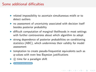
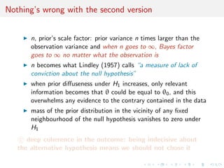
![Some further difficulties
long-lasting impact of prior modeling, i.e., choice of prior
distributions on parameters of both models, despite overall
consistency proof for Bayes factor
discontinuity in valid use of improper priors since they are not
justified in most testing situations, leading to many alternative
and ad hoc solutions, where data is either used twice or split
in artificial ways [or further tortured into confession]
binary (accept vs. reject) outcome more suited for immediate
decision (if any) than for model evaluation, in connection with
rudimentary loss function [atavistic remain of
Neyman-Pearson formalism]](https://image.slidesharecdn.com/obayes15-170315170942/85/An-overview-of-Bayesian-testing-10-320.jpg)
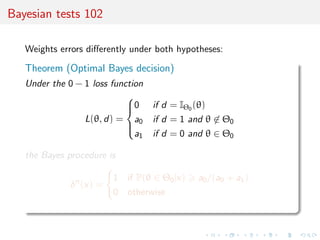
![Bayesian tests 101
Associated with the risk
R(θ, δ) = Eθ[L(θ, δ(x))]
=
Pθ(δ(x) = 0) if θ ∈ Θ0,
Pθ(δ(x) = 1) otherwise,
Bayes test
The Bayes estimator associated with π and with the 0 − 1 loss is
δπ
(x) =
1 if P(θ ∈ Θ0|x) > P(θ ∈ Θ0|x),
0 otherwise,](https://image.slidesharecdn.com/obayes15-170315170942/85/An-overview-of-Bayesian-testing-12-320.jpg)
![Bayesian tests 101
Associated with the risk
R(θ, δ) = Eθ[L(θ, δ(x))]
=
Pθ(δ(x) = 0) if θ ∈ Θ0,
Pθ(δ(x) = 1) otherwise,
Bayes test
The Bayes estimator associated with π and with the 0 − 1 loss is
δπ
(x) =
1 if P(θ ∈ Θ0|x) > P(θ ∈ Θ0|x),
0 otherwise,](https://image.slidesharecdn.com/obayes15-170315170942/85/An-overview-of-Bayesian-testing-13-320.jpg)
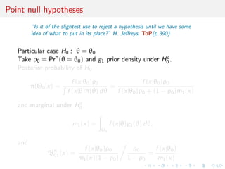
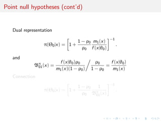
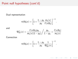
![A function of posterior probabilities
Definition (Bayes factors)
For hypotheses H0 : θ ∈ Θ0 vs. Ha : θ ∈ Θ0
B01 =
π(Θ0|x)
π(Θc
0|x)
π(Θ0)
π(Θc
0)
=
Θ0
f (x|θ)π0(θ)dθ
Θc
0
f (x|θ)π1(θ)dθ
[Jeffreys, ToP, 1939, V, §5.01]
Bayes rule under 0 − 1 loss: acceptance if
B01 > {(1 − π(Θ0))/a1}/{π(Θ0)/a0}](https://image.slidesharecdn.com/obayes15-170315170942/85/An-overview-of-Bayesian-testing-16-320.jpg)
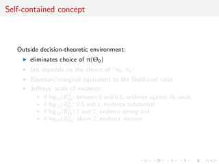
![self-contained concept
Outside decision-theoretic environment:
eliminates choice of π(Θ0)
but depends on the choice of (π0, π1)
Bayesian/marginal equivalent to the likelihood ratio
Jeffreys’ scale of evidence:
if log10(Bπ
10) between 0 and 0.5, evidence against H0 weak,
if log10(Bπ
10) 0.5 and 1, evidence substantial,
if log10(Bπ
10) 1 and 2, evidence strong and
if log10(Bπ
10) above 2, evidence decisive
[...fairly arbitrary!]](https://image.slidesharecdn.com/obayes15-170315170942/85/An-overview-of-Bayesian-testing-17-320.jpg)
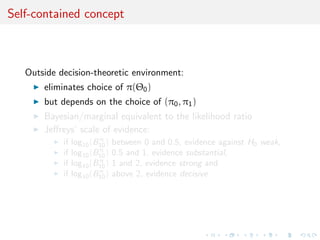
![self-contained concept
Outside decision-theoretic environment:
eliminates choice of π(Θ0)
but depends on the choice of (π0, π1)
Bayesian/marginal equivalent to the likelihood ratio
Jeffreys’ scale of evidence:
if log10(Bπ
10) between 0 and 0.5, evidence against H0 weak,
if log10(Bπ
10) 0.5 and 1, evidence substantial,
if log10(Bπ
10) 1 and 2, evidence strong and
if log10(Bπ
10) above 2, evidence decisive
[...fairly arbitrary!]](https://image.slidesharecdn.com/obayes15-170315170942/85/An-overview-of-Bayesian-testing-18-320.jpg)
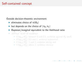
![self-contained concept
Outside decision-theoretic environment:
eliminates choice of π(Θ0)
but depends on the choice of (π0, π1)
Bayesian/marginal equivalent to the likelihood ratio
Jeffreys’ scale of evidence:
if log10(Bπ
10) between 0 and 0.5, evidence against H0 weak,
if log10(Bπ
10) 0.5 and 1, evidence substantial,
if log10(Bπ
10) 1 and 2, evidence strong and
if log10(Bπ
10) above 2, evidence decisive
[...fairly arbitrary!]](https://image.slidesharecdn.com/obayes15-170315170942/85/An-overview-of-Bayesian-testing-19-320.jpg)
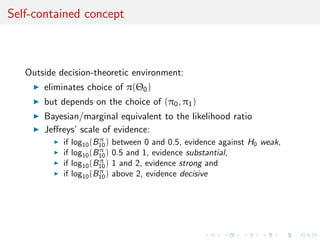
![self-contained concept
Outside decision-theoretic environment:
eliminates choice of π(Θ0)
but depends on the choice of (π0, π1)
Bayesian/marginal equivalent to the likelihood ratio
Jeffreys’ scale of evidence:
if log10(Bπ
10) between 0 and 0.5, evidence against H0 weak,
if log10(Bπ
10) 0.5 and 1, evidence substantial,
if log10(Bπ
10) 1 and 2, evidence strong and
if log10(Bπ
10) above 2, evidence decisive
[...fairly arbitrary!]](https://image.slidesharecdn.com/obayes15-170315170942/85/An-overview-of-Bayesian-testing-20-320.jpg)
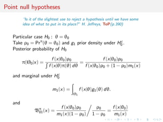
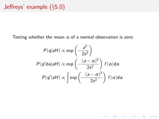
![Fundamental setting
Is the new parameter supported by the observations or is
any variation expressible by it better interpreted as
random? Thus we must set two hypotheses for
comparison, the more complicated having the smaller
initial probability (Jeffreys, ToP, V, §5.0)
...compare a specially suggested value of a new
parameter, often 0 [q], with the aggregate of other
possible values [q ]. We shall call q the null hypothesis
and q the alternative hypothesis [and] we must take
P(q|H) = P(q |H) = 1/2 .](https://image.slidesharecdn.com/obayes15-170315170942/85/An-overview-of-Bayesian-testing-25-320.jpg)
![Type–one and type–two errors
Associated with the risk
R(θ, δ) = Eθ[L(θ, δ(x))]
=
Pθ(δ(x) = 0) if θ ∈ Θ0,
Pθ(δ(x) = 1) otherwise,
Theorem (Bayes test)
The Bayes estimator associated with π and with the 0 − 1 loss is
δπ
(x) =
1 if P(θ ∈ Θ0|x) > P(θ ∈ Θ0|x),
0 otherwise,](https://image.slidesharecdn.com/obayes15-170315170942/85/An-overview-of-Bayesian-testing-27-320.jpg)
![Type–one and type–two errors
Associated with the risk
R(θ, δ) = Eθ[L(θ, δ(x))]
=
Pθ(δ(x) = 0) if θ ∈ Θ0,
Pθ(δ(x) = 1) otherwise,
Theorem (Bayes test)
The Bayes estimator associated with π and with the 0 − 1 loss is
δπ
(x) =
1 if P(θ ∈ Θ0|x) > P(θ ∈ Θ0|x),
0 otherwise,](https://image.slidesharecdn.com/obayes15-170315170942/85/An-overview-of-Bayesian-testing-28-320.jpg)
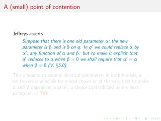
![Orthogonal parameters
If
I(α, β) =
gαα 0
0 gββ
,
α and β orthogonal, but not [a posteriori] independent, contrary to
ToP assertions
...the result will be nearly independent on previous
information on old parameters (V, §5.01).
and
K =
1
f (b, a)
ngββ
2π
exp −
1
2
ngββb2
[where] h(α) is irrelevant (V, §5.01)](https://image.slidesharecdn.com/obayes15-170315170942/85/An-overview-of-Bayesian-testing-32-320.jpg)
![Orthogonal parameters
If
I(α, β) =
gαα 0
0 gββ
,
α and β orthogonal, but not [a posteriori] independent, contrary to
ToP assertions
...the result will be nearly independent on previous
information on old parameters (V, §5.01).
and
K =
1
f (b, a)
ngββ
2π
exp −
1
2
ngββb2
[where] h(α) is irrelevant (V, §5.01)](https://image.slidesharecdn.com/obayes15-170315170942/85/An-overview-of-Bayesian-testing-33-320.jpg)
![A function of posterior probabilities
Definition (Bayes factors)
For hypotheses H0 : θ ∈ Θ0 vs. Ha : θ ∈ Θ0
B01 =
π(Θ0|x)
π(Θc
0|x)
π(Θ0)
π(Θc
0)
=
Θ0
f (x|θ)π0(θ)dθ
Θc
0
f (x|θ)π1(θ)dθ
[Good, 1958 & ToP, V, §5.01]
Equivalent to Bayes rule: acceptance if
B01 > {(1 − π(Θ0))/a1}/{π(Θ0)/a0}](https://image.slidesharecdn.com/obayes15-170315170942/85/An-overview-of-Bayesian-testing-39-320.jpg)
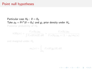
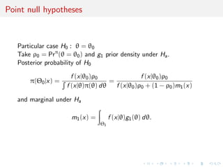
![A major modification
When the null hypothesis is supported by a set of measure 0
against Lebesgue measure, π(Θ0) = 0 for an absolutely continuous
prior distribution
[End of the story?!]
Suppose we are considering whether a location parameter
α is 0. The estimation prior probability for it is uniform
and we should have to take f (α) = 0 and K[= B10]
would always be infinite (V, §5.02)](https://image.slidesharecdn.com/obayes15-170315170942/85/An-overview-of-Bayesian-testing-44-320.jpg)
![A major modification
When the null hypothesis is supported by a set of measure 0
against Lebesgue measure, π(Θ0) = 0 for an absolutely continuous
prior distribution
[End of the story?!]
Suppose we are considering whether a location parameter
α is 0. The estimation prior probability for it is uniform
and we should have to take f (α) = 0 and K[= B10]
would always be infinite (V, §5.02)](https://image.slidesharecdn.com/obayes15-170315170942/85/An-overview-of-Bayesian-testing-45-320.jpg)
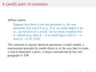
![ToP unaware of the problem?
A. Not entirely, as improper priors keep being used on nuisance
parameters
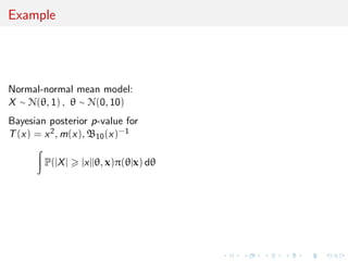
Example of testing for a zero normal mean:
If σ is the standard error and λ the true value, λ is 0 on
q. We want a suitable form for its prior on q . (...) Then
we should take
P(qdσ|H) ∝ dσ/σ
P(q dσdλ|H) ∝ f
λ
σ
dσ/σdλ/λ
where f [is a true density] (V, §5.2).
Fallacy of the “same” σ!](https://image.slidesharecdn.com/obayes15-170315170942/85/An-overview-of-Bayesian-testing-54-320.jpg)
![ToP unaware of the problem?
A. Not entirely, as improper priors keep being used on nuisance
parameters
Example of testing for a zero normal mean:
If σ is the standard error and λ the true value, λ is 0 on
q. We want a suitable form for its prior on q . (...) Then
we should take
P(qdσ|H) ∝ dσ/σ
P(q dσdλ|H) ∝ f
λ
σ
dσ/σdλ/λ
where f [is a true density] (V, §5.2).
Fallacy of the “same” σ!](https://image.slidesharecdn.com/obayes15-170315170942/85/An-overview-of-Bayesian-testing-55-320.jpg)
![Not enought information
If s = 0 [!!!], then [for σ = |¯x|/τ, λ = σv]
P(q|θH) ∝
∞
0
τ
|¯x|
n
exp −
1
2
nτ2 dτ
τ
,
P(q |θH) ∝
∞
0
dτ
τ
∞
−∞
τ
|¯x|
n
f (v) exp −
1
2
n(v − τ)2
.
If n = 1 and f (v) is any even [density],
P(q |θH) ∝
1
2
√
2π
|¯x|
and P(q|θH) ∝
1
2
√
2π
|¯x|
and therefore K = 1 (V, §5.2).](https://image.slidesharecdn.com/obayes15-170315170942/85/An-overview-of-Bayesian-testing-56-320.jpg)
![Strange constraints
If n 2, the condition that K = 0 for s = 0, ¯x = 0 is
equivalent to
∞
0
f (v)vn−1
dv = ∞ .
The function satisfying this condition for [all] n is
f (v) =
1
π(1 + v2)
This is the prior recommended by Jeffreys hereafter.
But, first, many other families of densities satisfy this constraint
and a scale of 1 cannot be universal!
Second, s = 0 is a zero probability event...](https://image.slidesharecdn.com/obayes15-170315170942/85/An-overview-of-Bayesian-testing-57-320.jpg)
![Strange constraints
If n 2, the condition that K = 0 for s = 0, ¯x = 0 is
equivalent to
∞
0
f (v)vn−1
dv = ∞ .
The function satisfying this condition for [all] n is
f (v) =
1
π(1 + v2)
This is the prior recommended by Jeffreys hereafter.
But, first, many other families of densities satisfy this constraint
and a scale of 1 cannot be universal!
Second, s = 0 is a zero probability event...](https://image.slidesharecdn.com/obayes15-170315170942/85/An-overview-of-Bayesian-testing-58-320.jpg)
![Strange constraints
If n 2, the condition that K = 0 for s = 0, ¯x = 0 is
equivalent to
∞
0
f (v)vn−1
dv = ∞ .
The function satisfying this condition for [all] n is
f (v) =
1
π(1 + v2)
This is the prior recommended by Jeffreys hereafter.
But, first, many other families of densities satisfy this constraint
and a scale of 1 cannot be universal!
Second, s = 0 is a zero probability event...](https://image.slidesharecdn.com/obayes15-170315170942/85/An-overview-of-Bayesian-testing-59-320.jpg)
![Comments
ToP very imprecise about choice of priors in the setting of
tests (despite existence of Susie’s Jeffreys’ conventional partly
proper priors)
ToP misses the difficulty of improper priors [coherent with
earlier stance]
but this problem still generates debates within the B
community
Some degree of goodness-of-fit testing but against fixed
alternatives
Persistence of the form
K ≈
πn
2
1 +
t2
ν
−1/2ν+1/2
but ν not so clearly defined...](https://image.slidesharecdn.com/obayes15-170315170942/85/An-overview-of-Bayesian-testing-60-320.jpg)
![what’s special about the Bayes factor?!
“The priors do not represent substantive knowledge of the
parameters within the model
Using Bayes’ theorem, these priors can then be updated to
posteriors conditioned on the data that were actually observed
In general, the fact that different priors result in different
Bayes factors should not come as a surprise
The Bayes factor (...) balances the tension between parsimony
and goodness of fit, (...) against overfitting the data
In induction there is no harm in being occasionally wrong; it is
inevitable that we shall be”
[Jeffreys, 1939; Ly et al., 2015]](https://image.slidesharecdn.com/obayes15-170315170942/85/An-overview-of-Bayesian-testing-62-320.jpg)
![what’s wrong with the Bayes factor?!
(1/2, 1/2) partition between hypotheses has very little to
suggest in terms of extensions
central difficulty stands with issue of picking a prior
probability of a model
unfortunate impossibility of using improper priors in most
settings
Bayes factors lack direct scaling associated with posterior
probability and loss function
twofold dependence on subjective prior measure, first in prior
weights of models and second in lasting impact of prior
modelling on the parameters
Bayes factor offers no window into uncertainty associated with
decision
further reasons in the summary
[Robert, 2016]](https://image.slidesharecdn.com/obayes15-170315170942/85/An-overview-of-Bayesian-testing-63-320.jpg)
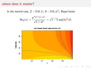
![Lindley’s paradox
In a normal mean testing problem,
¯xn ∼ N(θ, σ2
/n) , H0 : θ = θ0 ,
under Jeffreys prior, θ ∼ N(θ0, σ2), the Bayes factor
B01(tn) = (1 + n)1/2
exp −nt2
n/2[1 + n] ,
where tn =
√
n|¯xn − θ0|/σ, satisfies
B01(tn)
n−→∞
−→ ∞
[assuming a fixed tn]
[Lindley, 1957]](https://image.slidesharecdn.com/obayes15-170315170942/85/An-overview-of-Bayesian-testing-64-320.jpg)
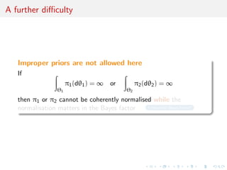
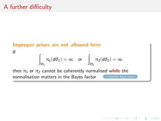
![A strong impropriety
Improper priors not allowed in Bayes factors:
If
Θ1
π1(dθ1) = ∞ or
Θ2
π2(dθ2) = ∞
then π1 or π2 cannot be coherently normalised while the
normalisation matters in the Bayes factor B12
Lack of mathematical justification for “common nuisance
parameter” [and prior of]
[Berger, Pericchi, and Varshavsky, 1998; Marin and Robert, 2013]](https://image.slidesharecdn.com/obayes15-170315170942/85/An-overview-of-Bayesian-testing-65-320.jpg)
![A strong impropriety
Improper priors not allowed in Bayes factors:
If
Θ1
π1(dθ1) = ∞ or
Θ2
π2(dθ2) = ∞
then π1 or π2 cannot be coherently normalised while the
normalisation matters in the Bayes factor B12
Lack of mathematical justification for “common nuisance
parameter” [and prior of]
[Berger, Pericchi, and Varshavsky, 1998; Marin and Robert, 2013]](https://image.slidesharecdn.com/obayes15-170315170942/85/An-overview-of-Bayesian-testing-66-320.jpg)
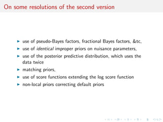
![On some resolutions of the paradox
use of pseudo-Bayes factors, fractional Bayes factors, &tc,
which lacks complete proper Bayesian justification
[Berger & Pericchi, 2001]
use of identical improper priors on nuisance parameters,
calibration via the posterior predictive distribution,
matching priors,
use of score functions extending the log score function
non-local priors correcting default priors](https://image.slidesharecdn.com/obayes15-170315170942/85/An-overview-of-Bayesian-testing-67-320.jpg)
![On some resolutions of the paradox
use of pseudo-Bayes factors, fractional Bayes factors, &tc,
use of identical improper priors on nuisance parameters, a
notion already entertained by Jeffreys
[Berger et al., 1998; Marin & Robert, 2013]
calibration via the posterior predictive distribution,
matching priors,
use of score functions extending the log score function
non-local priors correcting default priors](https://image.slidesharecdn.com/obayes15-170315170942/85/An-overview-of-Bayesian-testing-68-320.jpg)
![On some resolutions of the paradox
use of pseudo-Bayes factors, fractional Bayes factors, &tc,
use of identical improper priors on nuisance parameters,
P´ech´e de jeunesse: equating the values of the prior densities
at the point-null value θ0,
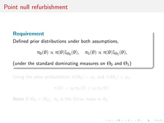
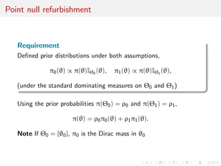
ρ0 = (1 − ρ0)π1(θ0)
[Robert, 1993]
calibration via the posterior predictive distribution,
matching priors,
use of score functions extending the log score function
non-local priors correcting default priors](https://image.slidesharecdn.com/obayes15-170315170942/85/An-overview-of-Bayesian-testing-69-320.jpg)
![On some resolutions of the paradox
use of pseudo-Bayes factors, fractional Bayes factors, &tc,
use of identical improper priors on nuisance parameters,
calibration via the posterior predictive distribution,
matching priors, whose sole purpose is to bring frequentist
and Bayesian coverages as close as possible
[Datta & Mukerjee, 2004]
use of score functions extending the log score function
non-local priors correcting default priors](https://image.slidesharecdn.com/obayes15-170315170942/85/An-overview-of-Bayesian-testing-71-320.jpg)
![On some resolutions of the paradox
use of pseudo-Bayes factors, fractional Bayes factors, &tc,
use of identical improper priors on nuisance parameters,
calibration via the posterior predictive distribution,
matching priors,
use of score functions extending the log score function
log B12(x) = log m1(x) − log m2(x) = S0(x, m1) − S0(x, m2) ,
that are independent of the normalising constant
[Dawid et al., 2013; Dawid & Musio, 2015]
non-local priors correcting default priors](https://image.slidesharecdn.com/obayes15-170315170942/85/An-overview-of-Bayesian-testing-72-320.jpg)
![On some resolutions of the paradox
use of pseudo-Bayes factors, fractional Bayes factors, &tc,
use of identical improper priors on nuisance parameters,
calibration via the posterior predictive distribution,
matching priors,
use of score functions extending the log score function
non-local priors correcting default priors towards more
balanced error rates
[Johnson & Rossell, 2010; Consonni et al., 2013]](https://image.slidesharecdn.com/obayes15-170315170942/85/An-overview-of-Bayesian-testing-73-320.jpg)
![Pseudo-Bayes factors
Idea
Use one part x[i] of the data x to make the prior proper:
πi improper but πi (·|x[i]) proper
and
fi (x[n/i]|θi ) πi (θi |x[i])dθi
fj (x[n/i]|θj ) πj (θj |x[i])dθj
independent of normalizing constant
Use remaining x[n/i] to run test as if πj (θj |x[i]) is the true prior](https://image.slidesharecdn.com/obayes15-170315170942/85/An-overview-of-Bayesian-testing-74-320.jpg)
![Pseudo-Bayes factors
Idea
Use one part x[i] of the data x to make the prior proper:
πi improper but πi (·|x[i]) proper
and
fi (x[n/i]|θi ) πi (θi |x[i])dθi
fj (x[n/i]|θj ) πj (θj |x[i])dθj
independent of normalizing constant
Use remaining x[n/i] to run test as if πj (θj |x[i]) is the true prior](https://image.slidesharecdn.com/obayes15-170315170942/85/An-overview-of-Bayesian-testing-75-320.jpg)
![Pseudo-Bayes factors
Idea
Use one part x[i] of the data x to make the prior proper:
πi improper but πi (·|x[i]) proper
and
fi (x[n/i]|θi ) πi (θi |x[i])dθi
fj (x[n/i]|θj ) πj (θj |x[i])dθj
independent of normalizing constant
Use remaining x[n/i] to run test as if πj (θj |x[i]) is the true prior](https://image.slidesharecdn.com/obayes15-170315170942/85/An-overview-of-Bayesian-testing-76-320.jpg)
![Issues
depends on the choice of x[i]
many ways of combining pseudo-Bayes factors
AIBF = BN
ji
1
L
Bij (x[ ])
MIBF = BN
ji med[Bij (x[ ])]
GIBF = BN
ji exp
1
L
log Bij (x[ ])
not often an exact Bayes factor
and thus lacking inner coherence
B12 = B10B02 and B01 = 1/B10 .
[Berger & Pericchi, 1996]](https://image.slidesharecdn.com/obayes15-170315170942/85/An-overview-of-Bayesian-testing-80-320.jpg)
![Issues
depends on the choice of x[i]
many ways of combining pseudo-Bayes factors
AIBF = BN
ji
1
L
Bij (x[ ])
MIBF = BN
ji med[Bij (x[ ])]
GIBF = BN
ji exp
1
L
log Bij (x[ ])
not often an exact Bayes factor
and thus lacking inner coherence
B12 = B10B02 and B01 = 1/B10 .
[Berger & Pericchi, 1996]](https://image.slidesharecdn.com/obayes15-170315170942/85/An-overview-of-Bayesian-testing-81-320.jpg)
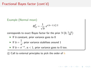
![Fractional Bayes factor
Idea
use directly the likelihood to separate training sample from testing
sample
BF
12 = B12(x)
Lb
2(θ2)π2(θ2)dθ2
Lb
1(θ1)π1(θ1)dθ1
[O’Hagan, 1995]
Proportion b of the sample used to gain proper-ness](https://image.slidesharecdn.com/obayes15-170315170942/85/An-overview-of-Bayesian-testing-82-320.jpg)
![Fractional Bayes factor
Idea
use directly the likelihood to separate training sample from testing
sample
BF
12 = B12(x)
Lb
2(θ2)π2(θ2)dθ2
Lb
1(θ1)π1(θ1)dθ1
[O’Hagan, 1995]
Proportion b of the sample used to gain proper-ness](https://image.slidesharecdn.com/obayes15-170315170942/85/An-overview-of-Bayesian-testing-83-320.jpg)

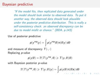
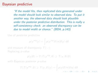
![Issues
“the posterior predictive p-value is such a [Bayesian]
probability statement, conditional on the model and data,
about what might be expected in future replications.
(BDA, p.151)
sounds too much like a p-value...!
relies on choice of T(·, ·)
seems to favour overfitting
(again) using the data twice (once for the posterior and twice
in the p-value)
needs to be calibrated (back to 0.05?)
general difficulty in interpreting
where is the penalty for model complexity?](https://image.slidesharecdn.com/obayes15-170315170942/85/An-overview-of-Bayesian-testing-87-320.jpg)
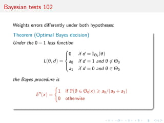
![Lindley’s paradox
In a normal mean testing problem,
¯xn ∼ N(θ, σ2
/n) , H0 : θ = θ0 ,
under Jeffreys prior, θ ∼ N(θ0, σ2), the Bayes factor
B01(tn) = (1 + n)1/2
exp −nt2
n/2[1 + n] ,
where tn =
√
n|¯xn − θ0|/σ, satisfies
B01(tn)
n−→∞
−→ ∞
[assuming a fixed tn]
[Lindley, 1957]](https://image.slidesharecdn.com/obayes15-170315170942/85/An-overview-of-Bayesian-testing-89-320.jpg)
![Two versions of the paradox
“the weight of Lindley’s paradoxical result (...) burdens
proponents of the Bayesian practice”.
[Lad, 2003]
official version, opposing frequentist and Bayesian assessments
[Lindley, 1957]
intra-Bayesian version, blaming vague and improper priors for
the Bayes factor misbehaviour:
if π1(·|σ) depends on a scale parameter σ, it is often the case
that
B01(x)
σ−→∞
−→ +∞
for a given x, meaning H0 is always accepted
[Robert, 1992, 2013]](https://image.slidesharecdn.com/obayes15-170315170942/85/An-overview-of-Bayesian-testing-90-320.jpg)
![Evacuation of the first version
Two paradigms [(b) versus (f)]
one (b) operates on the parameter space Θ, while the other
(f) is produced from the sample space
one (f) relies solely on the point-null hypothesis H0 and the
corresponding sampling distribution, while the other
(b) opposes H0 to a (predictive) marginal version of H1
one (f) could reject “a hypothesis that may be true (...)
because it has not predicted observable results that have not
occurred” (Jeffreys, ToP, VII, §7.2) while the other
(b) conditions upon the observed value xobs
one (f) cannot agree with the likelihood principle, while the
other (b) is almost uniformly in agreement with it
one (f) resorts to an arbitrary fixed bound α on the p-value,
while the other (b) refers to the (default) boundary probability
of 1/2](https://image.slidesharecdn.com/obayes15-170315170942/85/An-overview-of-Bayesian-testing-92-320.jpg)
![On some resolutions of the second version
use of pseudo-Bayes factors, fractional Bayes factors, &tc,
which lacks complete proper Bayesian justification
[Berger & Pericchi, 2001]
use of identical improper priors on nuisance parameters,
use of the posterior predictive distribution,
matching priors,
use of score functions extending the log score function
non-local priors correcting default priors](https://image.slidesharecdn.com/obayes15-170315170942/85/An-overview-of-Bayesian-testing-95-320.jpg)
![On some resolutions of the second version
use of pseudo-Bayes factors, fractional Bayes factors, &tc,
use of identical improper priors on nuisance parameters, a
notion already entertained by Jeffreys
[Berger et al., 1998; Marin & Robert, 2013]
use of the posterior predictive distribution,
matching priors,
use of score functions extending the log score function
non-local priors correcting default priors](https://image.slidesharecdn.com/obayes15-170315170942/85/An-overview-of-Bayesian-testing-96-320.jpg)
![On some resolutions of the second version
use of pseudo-Bayes factors, fractional Bayes factors, &tc,
use of identical improper priors on nuisance parameters,
P´ech´e de jeunesse: equating the values of the prior densities
at the point-null value θ0,
ρ0 = (1 − ρ0)π1(θ0)
[Robert, 1993]
use of the posterior predictive distribution,
matching priors,
use of score functions extending the log score function
non-local priors correcting default priors](https://image.slidesharecdn.com/obayes15-170315170942/85/An-overview-of-Bayesian-testing-97-320.jpg)
![On some resolutions of the second version
use of pseudo-Bayes factors, fractional Bayes factors, &tc,
use of identical improper priors on nuisance parameters,
use of the posterior predictive distribution,
matching priors, whose sole purpose is to bring frequentist
and Bayesian coverages as close as possible
[Datta & Mukerjee, 2004]
use of score functions extending the log score function
non-local priors correcting default priors](https://image.slidesharecdn.com/obayes15-170315170942/85/An-overview-of-Bayesian-testing-99-320.jpg)
![On some resolutions of the second version
use of pseudo-Bayes factors, fractional Bayes factors, &tc,
use of identical improper priors on nuisance parameters,
use of the posterior predictive distribution,
matching priors,
use of score functions extending the log score function
log B12(x) = log m1(x) − log m2(x) = S0(x, m1) − S0(x, m2) ,
that are independent of the normalising constant
[Dawid et al., 2013; Dawid & Musio, 2015]
non-local priors correcting default priors](https://image.slidesharecdn.com/obayes15-170315170942/85/An-overview-of-Bayesian-testing-100-320.jpg)
![On some resolutions of the second version
use of pseudo-Bayes factors, fractional Bayes factors, &tc,
use of identical improper priors on nuisance parameters,
use of the posterior predictive distribution,
matching priors,
use of score functions extending the log score function
non-local priors correcting default priors towards more
balanced error rates
[Johnson & Rossell, 2010; Consonni et al., 2013]](https://image.slidesharecdn.com/obayes15-170315170942/85/An-overview-of-Bayesian-testing-101-320.jpg)
![DIC as in Dayesian?
Deviance defined by
D(θ) = −2 log(p(y|θ)) ,
Effective number of parameters computed as
pD = ¯D − D(¯θ) ,
with ¯D posterior expectation of D and ¯θ estimate of θ
Deviance information criterion (DIC) defined by
DIC = pD + ¯D
= D(¯θ) + 2pD
Models with smaller DIC better supported by the data
[Spiegelhalter et al., 2002]](https://image.slidesharecdn.com/obayes15-170315170942/85/An-overview-of-Bayesian-testing-103-320.jpg)
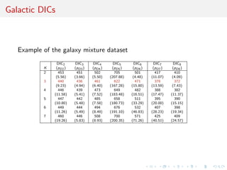
![how many DICs can you fit in a mixture?
Q: How many giraffes can you fit in a VW bug?
A: None, the elephants are in there.
1. observed DICs
DIC1 = −4Eθ [log f (y|θ)|y] + 2 log f (y|Eθ [θ|y])
often a poor choice in case of unidentifiability
2. complete DICs based on f (y, z|θ)
3. conditional DICs based on f (y|z, θ)
[Celeux et al., BA, 2006]](https://image.slidesharecdn.com/obayes15-170315170942/85/An-overview-of-Bayesian-testing-107-320.jpg)
![how many DICs can you fit in a mixture?
Q: How many giraffes can you fit in a VW bug?
A: None, the elephants are in there.
1. observed DICs
DIC2 = −4Eθ [log f (y|θ)|y] + 2 log f (y|θ(y)) .
which uses posterior mode instead
2. complete DICs based on f (y, z|θ)
3. conditional DICs based on f (y|z, θ)
[Celeux et al., BA, 2006]](https://image.slidesharecdn.com/obayes15-170315170942/85/An-overview-of-Bayesian-testing-108-320.jpg)
![how many DICs can you fit in a mixture?
Q: How many giraffes can you fit in a VW bug?
A: None, the elephants are in there.
1. observed DICs
DIC3 = −4Eθ [log f (y|θ)|y] + 2 log f (y) ,
which instead relies on the MCMC density estimate
2. complete DICs based on f (y, z|θ)
3. conditional DICs based on f (y|z, θ)
[Celeux et al., BA, 2006]](https://image.slidesharecdn.com/obayes15-170315170942/85/An-overview-of-Bayesian-testing-109-320.jpg)
![how many DICs can you fit in a mixture?
Q: How many giraffes can you fit in a VW bug?
A: None, the elephants are in there.
1. observed DICs
2. complete DICs based on f (y, z|θ)
DIC4 = EZ [DIC(y, Z)|y]
= −4Eθ,Z [log f (y, Z|θ)|y] + 2EZ [log f (y, Z|Eθ[θ|y, Z])|y]
3. conditional DICs based on f (y|z, θ)
[Celeux et al., BA, 2006]](https://image.slidesharecdn.com/obayes15-170315170942/85/An-overview-of-Bayesian-testing-110-320.jpg)
![how many DICs can you fit in a mixture?
Q: How many giraffes can you fit in a VW bug?
A: None, the elephants are in there.
1. observed DICs
2. complete DICs based on f (y, z|θ)
DIC5 = −4Eθ,Z [log f (y, Z|θ)|y] + 2 log f (y, z(y)|θ(y)) ,
using Z as an additional parameter
3. conditional DICs based on f (y|z, θ)
[Celeux et al., BA, 2006]](https://image.slidesharecdn.com/obayes15-170315170942/85/An-overview-of-Bayesian-testing-111-320.jpg)
![how many DICs can you fit in a mixture?
Q: How many giraffes can you fit in a VW bug?
A: None, the elephants are in there.
1. observed DICs
2. complete DICs based on f (y, z|θ)
DIC6 = −4Eθ,Z [log f (y, Z|θ)|y]+2EZ[log f (y, Z|θ(y))|y, θ(y)] .
in analogy with EM, θ being an EM fixed point
3. conditional DICs based on f (y|z, θ)
[Celeux et al., BA, 2006]](https://image.slidesharecdn.com/obayes15-170315170942/85/An-overview-of-Bayesian-testing-112-320.jpg)
![how many DICs can you fit in a mixture?
Q: How many giraffes can you fit in a VW bug?
A: None, the elephants are in there.
1. observed DICs
2. complete DICs based on f (y, z|θ)
3. conditional DICs based on f (y|z, θ)
DIC7 = −4Eθ,Z [log f (y|Z, θ)|y] + 2 log f (y|z(y), θ(y)) ,
using MAP estimates
[Celeux et al., BA, 2006]](https://image.slidesharecdn.com/obayes15-170315170942/85/An-overview-of-Bayesian-testing-113-320.jpg)
![how many DICs can you fit in a mixture?
Q: How many giraffes can you fit in a VW bug?
A: None, the elephants are in there.
1. observed DICs
2. complete DICs based on f (y, z|θ)
3. conditional DICs based on f (y|z, θ)
DIC8 = −4Eθ,Z [log f (y|Z, θ)|y]+2EZ log f (y|Z, θ(y, Z))|y ,
conditioning first on Z and then integrating over Z
conditional on y
[Celeux et al., BA, 2006]](https://image.slidesharecdn.com/obayes15-170315170942/85/An-overview-of-Bayesian-testing-114-320.jpg)
![questions
what is the behaviour of DIC under model mispecification?
is there an absolute scale to the DIC values, i.e. when is a
difference in DICs significant?
how can DIC handle small n’s versus p’s?
should pD be defined as var(D|y)/2 [Gelman’s suggestion]?
is WAIC (Gelman and Vehtari, 2013) making a difference for
being based on expected posterior predictive?
In an era of complex models, is DIC applicable?
[Robert, 2013]](https://image.slidesharecdn.com/obayes15-170315170942/85/An-overview-of-Bayesian-testing-116-320.jpg)
![questions
what is the behaviour of DIC under model mispecification?
is there an absolute scale to the DIC values, i.e. when is a
difference in DICs significant?
how can DIC handle small n’s versus p’s?
should pD be defined as var(D|y)/2 [Gelman’s suggestion]?
is WAIC (Gelman and Vehtari, 2013) making a difference for
being based on expected posterior predictive?
In an era of complex models, is DIC applicable?
[Robert, 2013]](https://image.slidesharecdn.com/obayes15-170315170942/85/An-overview-of-Bayesian-testing-117-320.jpg)
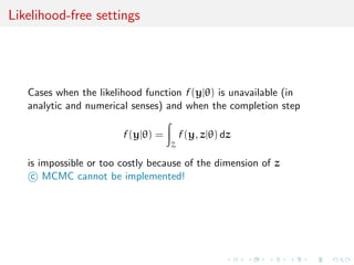
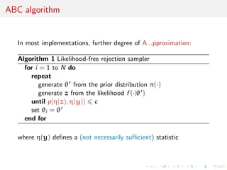
![The ABC method
Bayesian setting: target is π(θ)f (x|θ)
When likelihood f (x|θ) not in closed form, likelihood-free rejection
technique:
ABC algorithm
For an observation y ∼ f (y|θ), under the prior π(θ), keep jointly
simulating
θ ∼ π(θ) , z ∼ f (z|θ ) ,
until the auxiliary variable z is equal to the observed value, z = y.
[Tavar´e et al., 1997]](https://image.slidesharecdn.com/obayes15-170315170942/85/An-overview-of-Bayesian-testing-120-320.jpg)
![The ABC method
Bayesian setting: target is π(θ)f (x|θ)
When likelihood f (x|θ) not in closed form, likelihood-free rejection
technique:
ABC algorithm
For an observation y ∼ f (y|θ), under the prior π(θ), keep jointly
simulating
θ ∼ π(θ) , z ∼ f (z|θ ) ,
until the auxiliary variable z is equal to the observed value, z = y.
[Tavar´e et al., 1997]](https://image.slidesharecdn.com/obayes15-170315170942/85/An-overview-of-Bayesian-testing-121-320.jpg)
![The ABC method
Bayesian setting: target is π(θ)f (x|θ)
When likelihood f (x|θ) not in closed form, likelihood-free rejection
technique:
ABC algorithm
For an observation y ∼ f (y|θ), under the prior π(θ), keep jointly
simulating
θ ∼ π(θ) , z ∼ f (z|θ ) ,
until the auxiliary variable z is equal to the observed value, z = y.
[Tavar´e et al., 1997]](https://image.slidesharecdn.com/obayes15-170315170942/85/An-overview-of-Bayesian-testing-122-320.jpg)
![A as A...pproximative
When y is a continuous random variable, strict equality z = y is
replaced with a tolerance zone
ρ(y, z)
where ρ is a distance
Output distributed from
π(θ) Pθ{ρ(y, z) < }
def
∝ π(θ|ρ(y, z) < )
[Pritchard et al., 1999]](https://image.slidesharecdn.com/obayes15-170315170942/85/An-overview-of-Bayesian-testing-123-320.jpg)
![A as A...pproximative
When y is a continuous random variable, strict equality z = y is
replaced with a tolerance zone
ρ(y, z)
where ρ is a distance
Output distributed from
π(θ) Pθ{ρ(y, z) < }
def
∝ π(θ|ρ(y, z) < )
[Pritchard et al., 1999]](https://image.slidesharecdn.com/obayes15-170315170942/85/An-overview-of-Bayesian-testing-124-320.jpg)
![Which summary η(·)?
Fundamental difficulty of the choice of the summary statistic when
there is no non-trivial sufficient statistics
Loss of statistical information balanced against gain in data
roughening
Approximation error and information loss remain unknown
Choice of statistics induces choice of distance function
towards standardisation
may be imposed for external/practical reasons (e.g., LDA)
may gather several non-B point estimates
can learn about efficient combination
[Estoup et al., 2012, Genetics]](https://image.slidesharecdn.com/obayes15-170315170942/85/An-overview-of-Bayesian-testing-126-320.jpg)
![Which summary η(·)?
Fundamental difficulty of the choice of the summary statistic when
there is no non-trivial sufficient statistics
Loss of statistical information balanced against gain in data
roughening
Approximation error and information loss remain unknown
Choice of statistics induces choice of distance function
towards standardisation
may be imposed for external/practical reasons (e.g., LDA)
may gather several non-B point estimates
can learn about efficient combination
[Estoup et al., 2012, Genetics]](https://image.slidesharecdn.com/obayes15-170315170942/85/An-overview-of-Bayesian-testing-127-320.jpg)
![Which summary η(·)?
Fundamental difficulty of the choice of the summary statistic when
there is no non-trivial sufficient statistics
Loss of statistical information balanced against gain in data
roughening
Approximation error and information loss remain unknown
Choice of statistics induces choice of distance function
towards standardisation
may be imposed for external/practical reasons (e.g., LDA)
may gather several non-B point estimates
can learn about efficient combination
[Estoup et al., 2012, Genetics]](https://image.slidesharecdn.com/obayes15-170315170942/85/An-overview-of-Bayesian-testing-128-320.jpg)
![Generic ABC for model choice
Algorithm 2 Likelihood-free model choice sampler (ABC-MC)
for t = 1 to T do
repeat
Generate m from the prior π(M = m)
Generate θm from the prior πm(θm)
Generate z from the model fm(z|θm)
until ρ{η(z), η(y)} <
Set m(t) = m and θ(t)
= θm
end for
[Grelaud et al., 2009]](https://image.slidesharecdn.com/obayes15-170315170942/85/An-overview-of-Bayesian-testing-129-320.jpg)
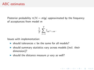
![ABC estimates
Posterior probability π(M = m|y) approximated by the frequency
of acceptances from model m
1
T
T
t=1
Im(t)=m .
Extension to a weighted polychotomous logistic regression estimate
of π(M = m|y), with non-parametric kernel weights
[Cornuet et al., DIYABC, 2009]](https://image.slidesharecdn.com/obayes15-170315170942/85/An-overview-of-Bayesian-testing-131-320.jpg)
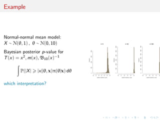
![A benchmark if toy example
Comparison suggested by referee of PNAS paper [thanks]:
[X, Cornuet, Marin, & Pillai, Aug. 2011]
Model M1: y ∼ N(θ1, 1) opposed to model M2: y ∼ L(θ2, 1/
√
2),
Laplace distribution with mean θ2 and scale parameter 1/
√
2
(variance one).](https://image.slidesharecdn.com/obayes15-170315170942/85/An-overview-of-Bayesian-testing-134-320.jpg)
![A benchmark if toy example
Comparison suggested by referee of PNAS paper [thanks]:
[X, Cornuet, Marin, & Pillai, Aug. 2011]
Model M1: y ∼ N(θ1, 1) opposed to model M2: y ∼ L(θ2, 1/
√
2),
Laplace distribution with mean θ2 and scale parameter 1/
√
2
(variance one).
Four possible statistics
1. sample mean y (sufficient for M1 if not M2);
2. sample median med(y) (insufficient);
3. sample variance var(y) (ancillary);
4. median absolute deviation mad(y) = med(y − med(y));](https://image.slidesharecdn.com/obayes15-170315170942/85/An-overview-of-Bayesian-testing-135-320.jpg)
![A benchmark if toy example
Comparison suggested by referee of PNAS paper [thanks]:
[X, Cornuet, Marin, & Pillai, Aug. 2011]
Model M1: y ∼ N(θ1, 1) opposed to model M2: y ∼ L(θ2, 1/
√
2),
Laplace distribution with mean θ2 and scale parameter 1/
√
2
(variance one).
0.0 0.2 0.4 0.6 0.8 1.0
0123
probability
Density](https://image.slidesharecdn.com/obayes15-170315170942/85/An-overview-of-Bayesian-testing-136-320.jpg)
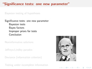
![A benchmark if toy example
Comparison suggested by referee of PNAS paper [thanks]:
[X, Cornuet, Marin, & Pillai, Aug. 2011]
Model M1: y ∼ N(θ1, 1) opposed to model M2: y ∼ L(θ2, 1/
√
2),
Laplace distribution with mean θ2 and scale parameter 1/
√
2
(variance one).
q
q
q
q
q
q
q
q
q
q
q
q
q
q
q
q
q
q
Gauss Laplace
0.00.20.40.60.81.0
n=100](https://image.slidesharecdn.com/obayes15-170315170942/85/An-overview-of-Bayesian-testing-137-320.jpg)
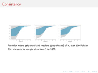
![Consistency theorem
If Pn belongs to one of the two models and if µ0 = E[T] cannot
be attained by the other one :
0 = min (inf{|µ0 − µi (θi )|; θi ∈ Θi }, i = 1, 2)
< max (inf{|µ0 − µi (θi )|; θi ∈ Θi }, i = 1, 2) ,
then the Bayes factor BT
12 is consistent](https://image.slidesharecdn.com/obayes15-170315170942/85/An-overview-of-Bayesian-testing-138-320.jpg)

![Issues
“the posterior predictive p-value is such a [Bayesian]
probability statement, conditional on the model and data,
about what might be expected in future replications.
(BDA, p.151)
sounds too much like a p-value...!
relies on choice of T(·, ·)
seems to favour overfitting
(again) using the data twice (once for the posterior and twice
in the p-value)
needs to be calibrated (back to 0.05?)
general difficulty in interpreting
where is the penalty for model complexity?](https://image.slidesharecdn.com/obayes15-170315170942/85/An-overview-of-Bayesian-testing-142-320.jpg)
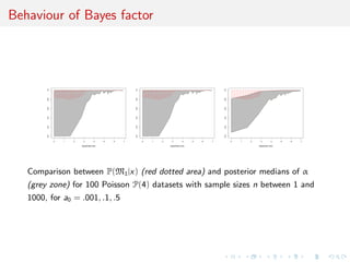
![goodness-of-fit [only?]
“A model is suspect if a discrepancy is of practical importance and
its observed value has a tail-area probability near 0 or 1, indicating
that the observed pattern would be unlikely to be seen in
replications of the data if the model were true. An extreme p-value
implies that the model cannot be expected to capture this aspect of
the data. A p-value is a posterior probability and can therefore be
interpreted directly—although not as Pr(model is true — data).
Major failures of the model (...) can be addressed by expanding the
model appropriately.” BDA, p.150
not helpful in comparing models (both may be deficient)
anti-Ockham? i.e., may favour larger dimensions (if prior
concentrated enough)
lingering worries about using the data twice and favourable
bias
impact of the prior (only under the current model) but allows
for improper priors](https://image.slidesharecdn.com/obayes15-170315170942/85/An-overview-of-Bayesian-testing-146-320.jpg)
![goodness-of-fit [only?]
“A model is suspect if a discrepancy is of practical importance and
its observed value has a tail-area probability near 0 or 1, indicating
that the observed pattern would be unlikely to be seen in
replications of the data if the model were true. An extreme p-value
implies that the model cannot be expected to capture this aspect of
the data. A p-value is a posterior probability and can therefore be
interpreted directly—although not as Pr(model is true — data).
Major failures of the model (...) can be addressed by expanding the
model appropriately.” BDA, p.150
not helpful in comparing models (both may be deficient)
anti-Ockham? i.e., may favour larger dimensions (if prior
concentrated enough)
lingering worries about using the data twice and favourable
bias
impact of the prior (only under the current model) but allows
for improper priors](https://image.slidesharecdn.com/obayes15-170315170942/85/An-overview-of-Bayesian-testing-147-320.jpg)
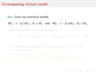
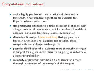
![Weakly informative motivations
using the same parameters or some identical parameters on
both components highlights that opposition between the two
components is not an issue of enjoying different parameters
those common parameters are nuisance parameters, to be
integrated out [unlike Lindley’s paradox]
prior model weights ωi rarely discussed in classical Bayesian
approach, even though linear impact on posterior probabilities.
Here, prior modeling only involves selecting a prior on α, e.g.,
α ∼ B(a0, a0)
while a0 impacts posterior on α, it always leads to mass
accumulation near 1 or 0, i.e. favours most likely model
sensitivity analysis straightforward to carry
approach easily calibrated by parametric boostrap providing
reference posterior of α under each model
natural Metropolis–Hastings alternative](https://image.slidesharecdn.com/obayes15-170315170942/85/An-overview-of-Bayesian-testing-158-320.jpg)
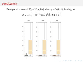
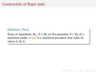
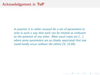
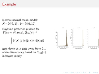
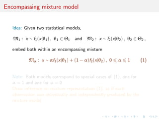
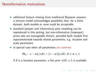
![Comparison with posterior probability
0 100 200 300 400 500
-50-40-30-20-100
a0=.1
sample size
0 100 200 300 400 500
-50-40-30-20-100
a0=.3
sample size
0 100 200 300 400 500
-50-40-30-20-100
a0=.4
sample size
0 100 200 300 400 500
-50-40-30-20-100
a0=.5
sample size
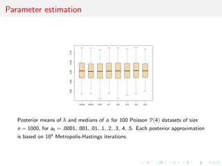
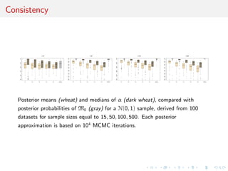
Plots of ranges of log(n) log(1 − E[α|x]) (gray color) and log(1 − p(M1|x)) (red
dotted) over 100 N(0, 1) samples as sample size n grows from 1 to 500. and α
is the weight of N(0, 1) in the mixture model. The shaded areas indicate the
range of the estimations and each plot is based on a Beta prior with
a0 = .1, .2, .3, .4, .5, 1 and each posterior approximation is based on 104
iterations.](https://image.slidesharecdn.com/obayes15-170315170942/85/An-overview-of-Bayesian-testing-171-320.jpg)
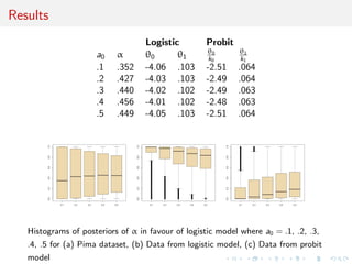
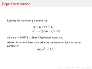
![Common parameterisation
Local reparameterisation strategy that rescales parameters of the
probit model M2 so that the MLE’s of both models coincide.
[Choudhuty et al., 2007]
Φ(xi
θ2) ≈
exp(kxi θ2)
1 + exp(kxi θ2)
and use best estimate of k to bring both parameters into coherency
(k0, k1) = (θ01/θ02, θ11/θ12) ,
reparameterise M1 and M2 as
M1 :yi | xi
, θ ∼ B(1, pi ) where pi =
exp(xi θ)
1 + exp(xi θ)
M2 :yi | xi
, θ ∼ B(1, qi ) where qi = Φ(xi
(κ−1
θ)) ,
with κ−1θ = (θ0/k0, θ1/k1).](https://image.slidesharecdn.com/obayes15-170315170942/85/An-overview-of-Bayesian-testing-174-320.jpg)
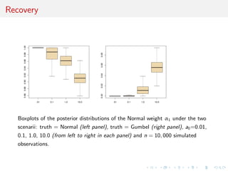
![Prior modelling
Under default g-prior
θ ∼ N2(0, n(XT
X)−1
)
full conditional posterior distributions given allocations
π(θ | y, X, ζ) ∝
exp i Iζi =1yi xi θ
i;ζi =1[1 + exp(xi θ)]
exp −θT
(XT
X)θ 2n
×
i;ζi =2
Φ(xi
(κ−1
θ))yi
(1 − Φ(xi
(κ−1
θ)))(1−yi )
hence posterior distribution clearly defined](https://image.slidesharecdn.com/obayes15-170315170942/85/An-overview-of-Bayesian-testing-175-320.jpg)
![Asymptotic consistency
Posterior consistency holds for mixture testing procedure [under
minor conditions]
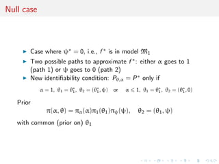
Two different cases
the two models, M1 and M2, are well separated
model M1 is a submodel of M2.](https://image.slidesharecdn.com/obayes15-170315170942/85/An-overview-of-Bayesian-testing-182-320.jpg)
![Asymptotic consistency
Posterior consistency holds for mixture testing procedure [under
minor conditions]
Two different cases
the two models, M1 and M2, are well separated
model M1 is a submodel of M2.](https://image.slidesharecdn.com/obayes15-170315170942/85/An-overview-of-Bayesian-testing-183-320.jpg)
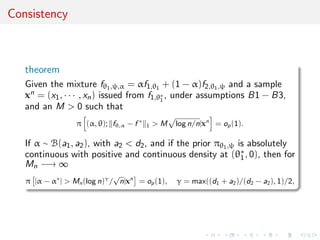
![Posterior concentration rate
Let π be the prior and xn = (x1, · · · , xn) a sample with true
density f ∗
proposition
Assume that, for all c > 0, there exist Θn ⊂ Θ1 × Θ2 and B > 0 such that
π [Θc
n] n−c
, Θn ⊂ { θ1 + θ2 nB
}
and that there exist H 0 and L, δ > 0 such that, for j = 1, 2,
sup
θ,θ ∈Θn
fj,θj
− fj,θj
1 LnH
θj − θj , θ = (θ1, θ2), θ = (θ1, θ2) ,
∀ θj − θ∗
j δ; KL(fj,θj
, fj,θ∗
j
) θj − θ∗
j .
Then, when f ∗
= fθ∗,α∗ , with α∗
∈ [0, 1], there exists M > 0 such that
π (α, θ); fθ,α − f ∗
1 > M log n/n|xn
= op(1) .](https://image.slidesharecdn.com/obayes15-170315170942/85/An-overview-of-Bayesian-testing-184-320.jpg)
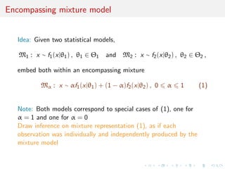
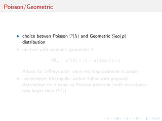
![Separated models
Assumption: Models are separated, i.e. identifiability holds:
∀α, α ∈ [0, 1], ∀θj , θj , j = 1, 2 Pθ,α = Pθ ,α ⇒ α = α , θ = θ
Further
inf
θ1∈Θ1
inf
θ2∈Θ2
f1,θ1
− f2,θ2 1 > 0
and, for θ∗
j ∈ Θj , if Pθj
weakly converges to Pθ∗
j
, then
θj −→ θ∗
j
in the Euclidean topology](https://image.slidesharecdn.com/obayes15-170315170942/85/An-overview-of-Bayesian-testing-185-320.jpg)
![Separated models
Assumption: Models are separated, i.e. identifiability holds:
∀α, α ∈ [0, 1], ∀θj , θj , j = 1, 2 Pθ,α = Pθ ,α ⇒ α = α , θ = θ
theorem
Under above assumptions, then for all > 0,
π [|α − α∗
| > |xn
] = op(1)](https://image.slidesharecdn.com/obayes15-170315170942/85/An-overview-of-Bayesian-testing-186-320.jpg)
![Separated models
Assumption: Models are separated, i.e. identifiability holds:
∀α, α ∈ [0, 1], ∀θj , θj , j = 1, 2 Pθ,α = Pθ ,α ⇒ α = α , θ = θ
theorem
If
θj → fj,θj
is C2 around θ∗
j , j = 1, 2,
f1,θ∗
1
− f2,θ∗
2
, f1,θ∗
1
, f2,θ∗
2
are linearly independent in y and
there exists δ > 0 such that
f1,θ∗
1
, f2,θ∗
2
, sup
|θ1−θ∗
1 |<δ
|D2
f1,θ1
|, sup
|θ2−θ∗
2 |<δ
|D2
f2,θ2
| ∈ L1
then
π |α − α∗
| > M log n/n xn
= op(1).](https://image.slidesharecdn.com/obayes15-170315170942/85/An-overview-of-Bayesian-testing-187-320.jpg)
![Separated models
Assumption: Models are separated, i.e. identifiability holds:
∀α, α ∈ [0, 1], ∀θj , θj , j = 1, 2 Pθ,α = Pθ ,α ⇒ α = α , θ = θ
theorem allows for interpretation of α under the posterior: If data
xn is generated from model M1 then posterior on α concentrates
around α = 1](https://image.slidesharecdn.com/obayes15-170315170942/85/An-overview-of-Bayesian-testing-188-320.jpg)
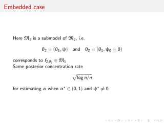
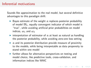
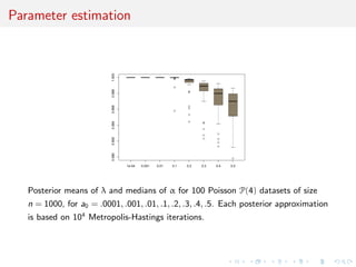
![Assumptions
[B1] Regularity: Assume that θ1 → f1,θ1 and θ2 → f2,θ2 are 3
times continuously differentiable and that
F∗
¯f 3
1,θ∗
1
f 3
1,θ∗
1
< +∞, ¯f1,θ∗
1
= sup
|θ1−θ∗
1 |<δ
f1,θ1
, f 1,θ∗
1
= inf
|θ1−θ∗
1 |<δ
f1,θ1
F∗
sup|θ1−θ∗
1 |<δ | f1,θ∗
1
|3
f 3
1,θ∗
1
< +∞, F∗
| f1,θ∗
1
|4
f 4
1,θ∗
1
< +∞,
F∗
sup|θ1−θ∗
1 |<δ |D2
f1,θ∗
1
|2
f 2
1,θ∗
1
< +∞, F∗
sup|θ1−θ∗
1 |<δ |D3
f1,θ∗
1
|
f 1,θ∗
1
< +∞](https://image.slidesharecdn.com/obayes15-170315170942/85/An-overview-of-Bayesian-testing-192-320.jpg)
![Assumptions
[B2] Integrability: There exists
S0 ⊂ S ∩ {|ψ| > δ0}
for some positive δ0 and satisfying Leb(S0) > 0, and such that for
all ψ ∈ S0,
F∗
sup|θ1−θ∗
1 |<δ f2,θ1,ψ
f 4
1,θ∗
1
< +∞, F∗
sup|θ1−θ∗
1 |<δ f 3
2,θ1,ψ
f 3
1,θ1∗
< +∞,](https://image.slidesharecdn.com/obayes15-170315170942/85/An-overview-of-Bayesian-testing-193-320.jpg)
![Assumptions
[B3] Stronger identifiability: Set
f2,θ∗
1,ψ∗ (x) = θ1 f2,θ∗
1,ψ∗ (x)T
, ψf2,θ∗
1,ψ∗ (x)T T
.
Then for all ψ ∈ S with ψ = 0, if η0 ∈ R, η1 ∈ Rd1
η0(f1,θ∗
1
− f2,θ∗
1,ψ) + ηT
1 θ1 f1,θ∗
1
= 0 ⇔ η1 = 0, η2 = 0](https://image.slidesharecdn.com/obayes15-170315170942/85/An-overview-of-Bayesian-testing-194-320.jpg)
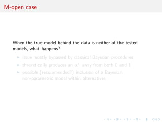
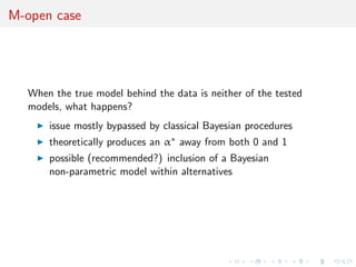
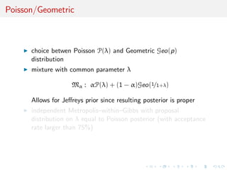
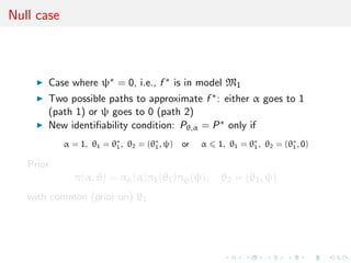
![Towards which decision?
And if we have to make a decision?
soft consider behaviour of posterior under prior predictives
or posterior predictive [e.g., prior predictive does not exist]
boostrapping behaviour
comparison with Bayesian non-parametric solution
hard rethink the loss function](https://image.slidesharecdn.com/obayes15-170315170942/85/An-overview-of-Bayesian-testing-198-320.jpg)

This document discusses several perspectives and solutions to Bayesian hypothesis testing. It outlines issues with Bayesian testing such as the dependence on prior distributions and difficulties interpreting Bayesian measures like posterior probabilities and Bayes factors. It discusses how Bayesian testing compares models rather than identifying a single true model. Several solutions to challenges are discussed, like using Bayes factors which eliminate the dependence on prior model probabilities but introduce other issues. The document also discusses testing under specific models like comparing a point null hypothesis to alternatives. Overall it presents both Bayesian and frequentist views on hypothesis testing and some of the open controversies in the field.