Download as PDF, PPTX
![Example of Bayes rule
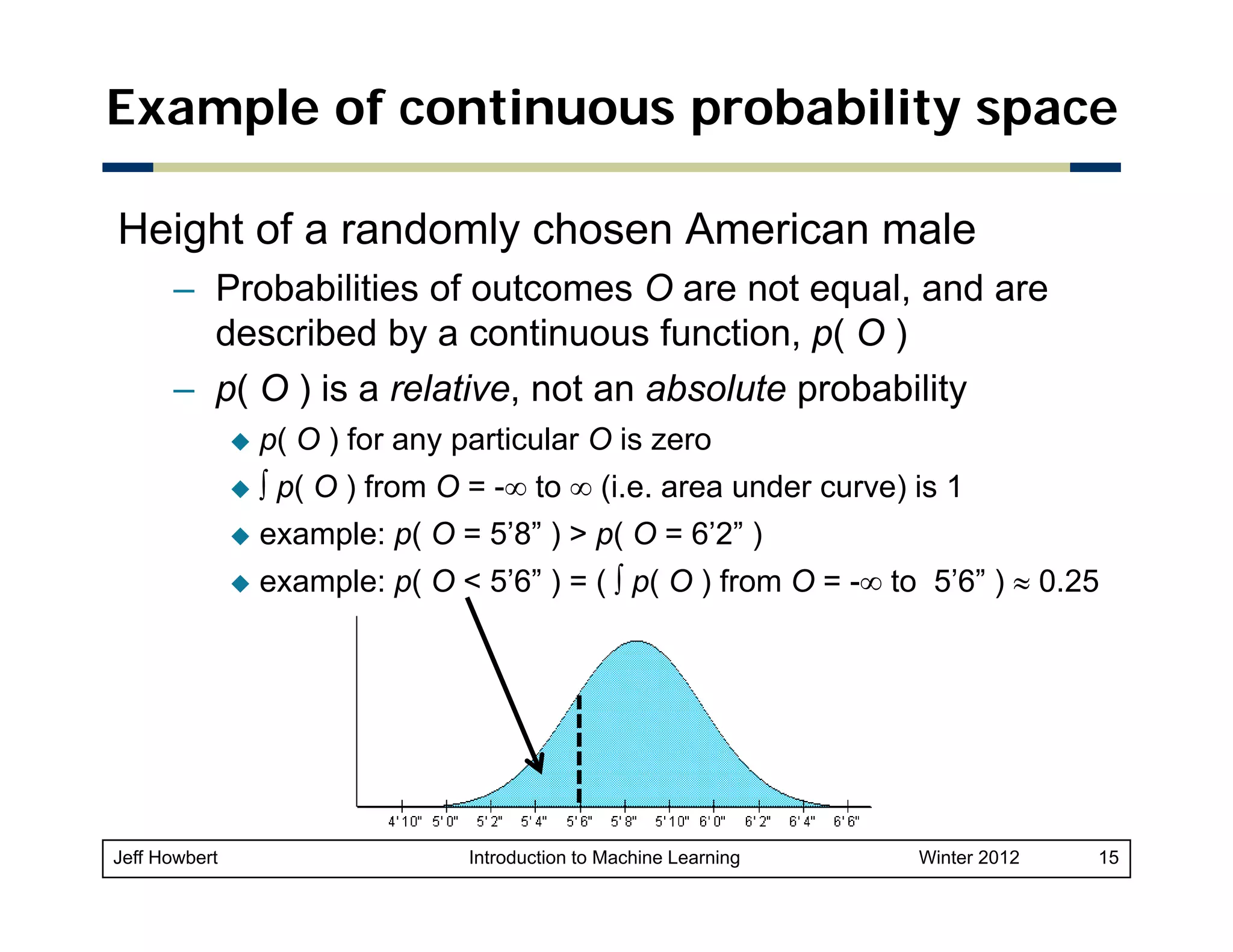
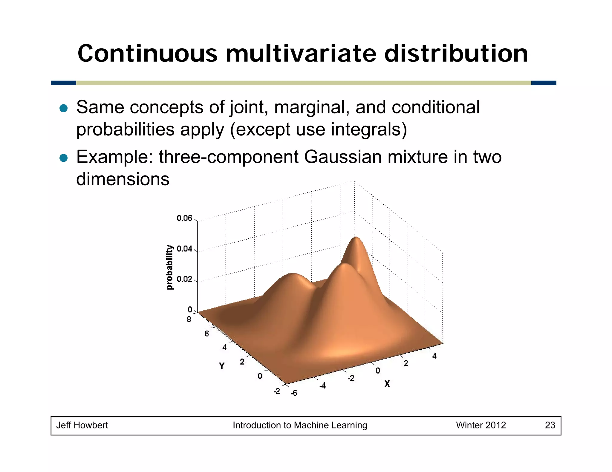
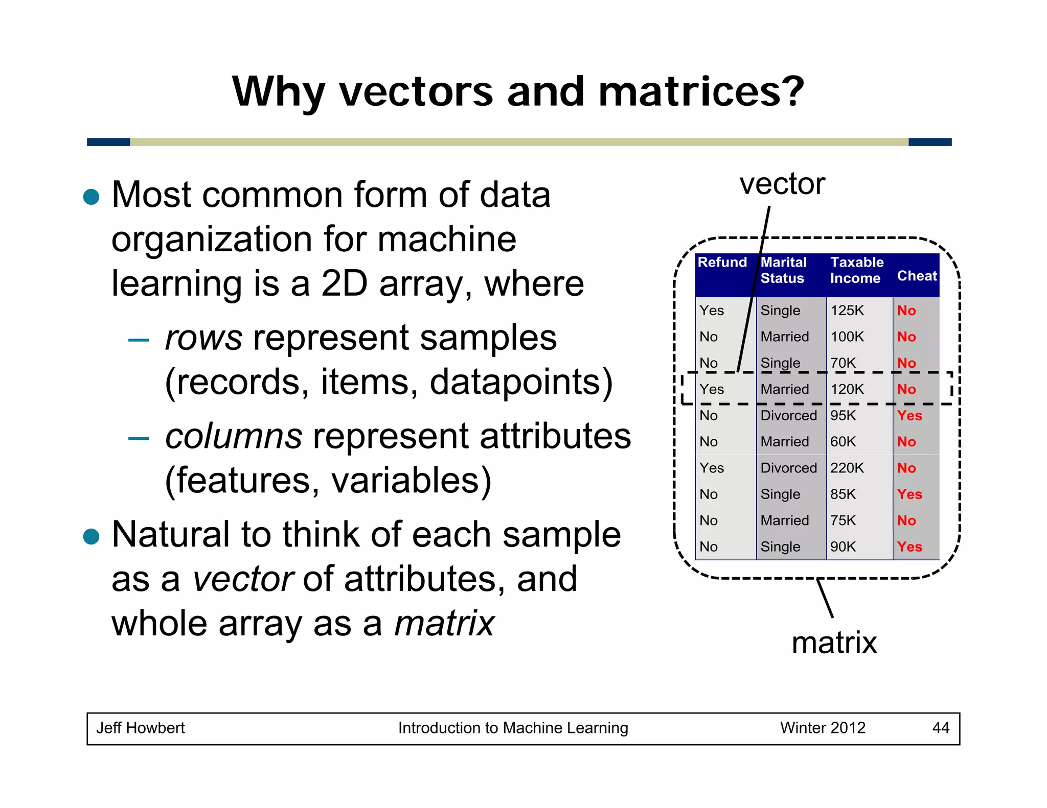
Marie is getting married tomorrow at an outdoor ceremony in the
desert. In recent years, it has rained only 5 days each year.
Unfortunately,
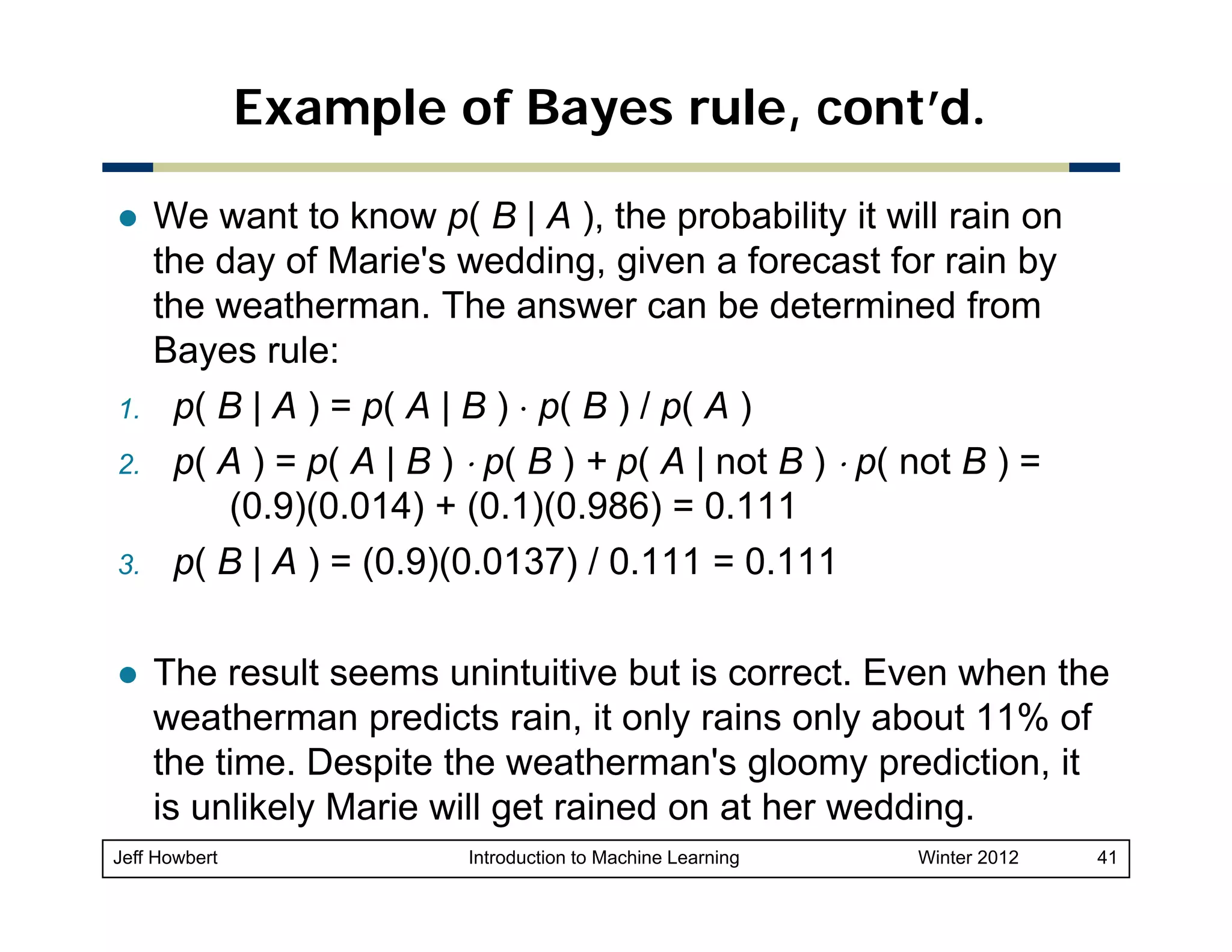
Unfortunately the weatherman is forecasting rain for tomorrow When
tomorrow.
it actually rains, the weatherman has forecast rain 90% of the time.
When it doesn't rain, he has forecast rain 10% of the time. What is the
probability it will rain on the day of Marie's wedding?
Marie s
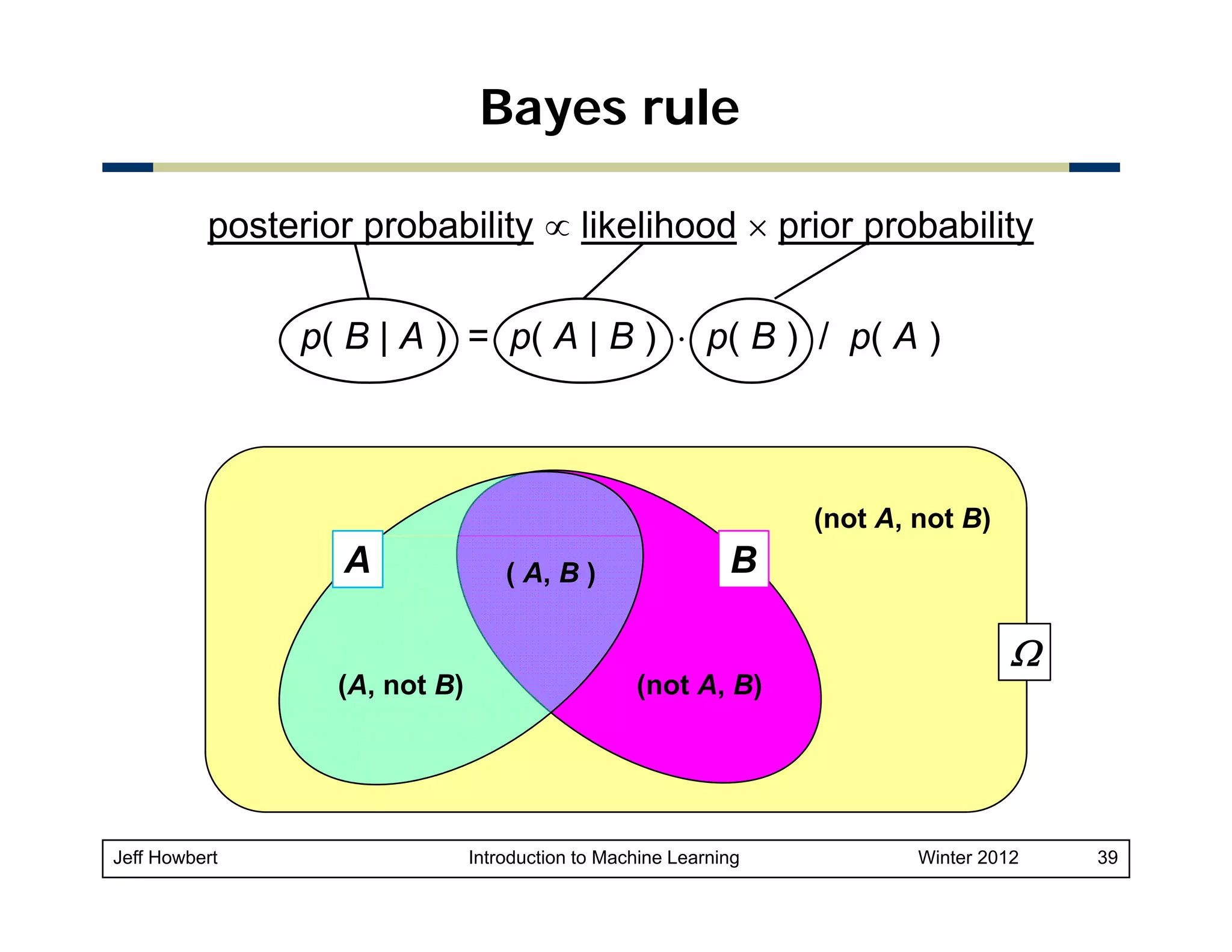
Event A: The weatherman has forecast rain.
Event B: It rains.
We know:
– p( B ) = 5 / 365 = 0.0137 [ It rains 5 days out of the year. ]
– p( not B ) = 360 / 365 = 0.9863
– p( A | B ) = 0.9 [ When it rains, the weatherman has forecast
rain 90% of the time. ]
– p( A | not B ) = 0.1 [When it does not rain the weatherman has
01
rain,
forecast rain 10% of the time.]
Jeff Howbert
Introduction to Machine Learning
Winter 2012
40](https://image.slidesharecdn.com/02mathessentials-140305011717-phpapp02/75/02-math-essentials-40-2048.jpg)
![Vector projection
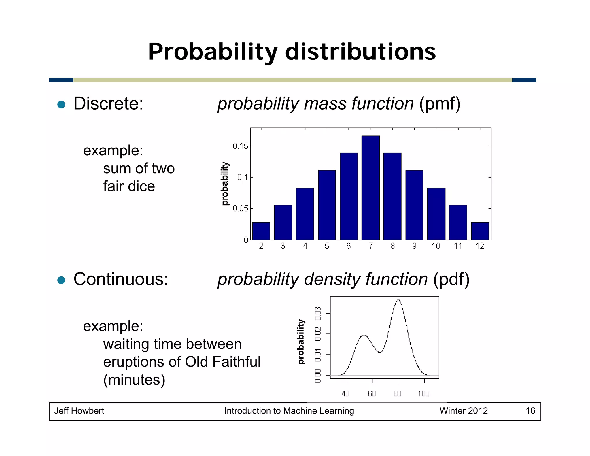
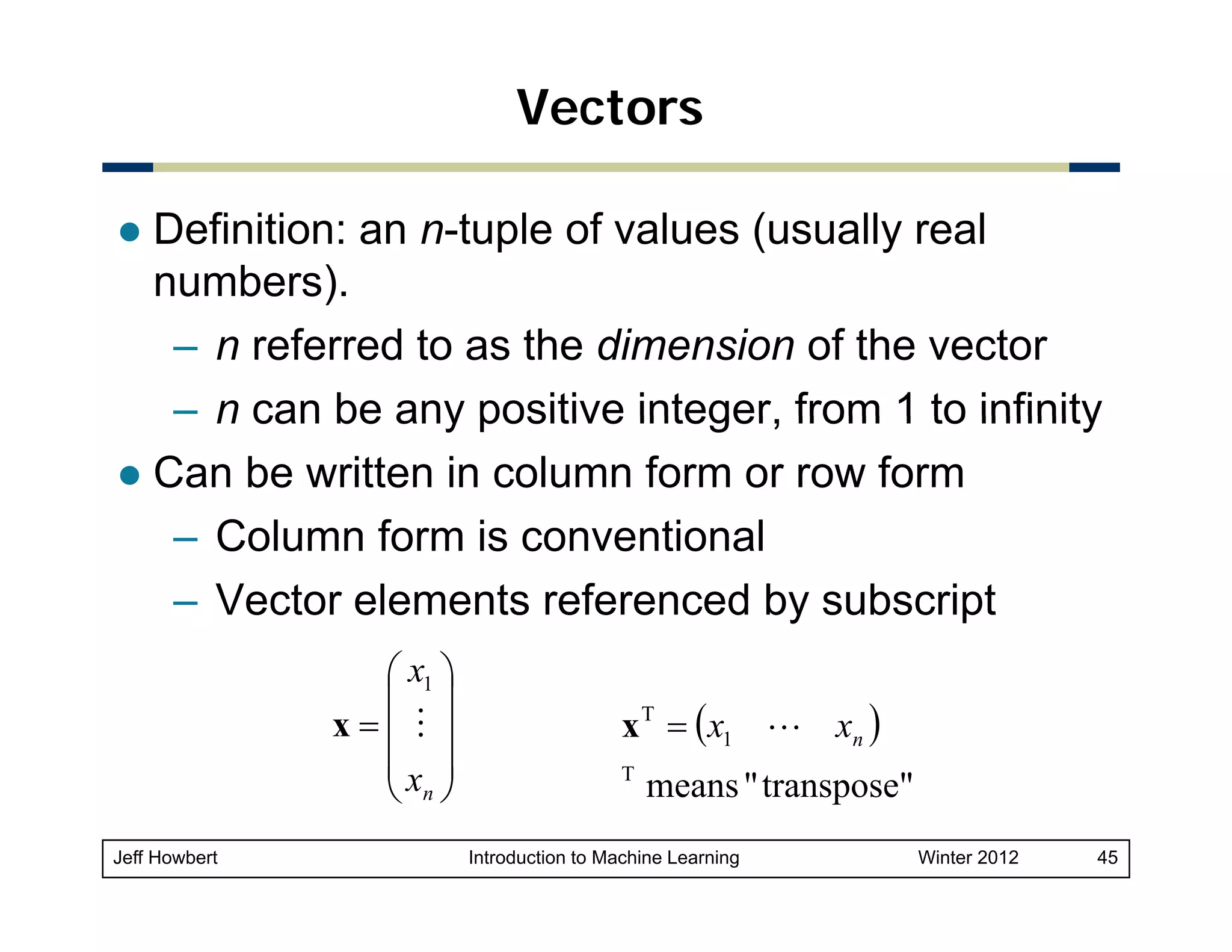
Orthogonal projection of y onto x
– Can take place in any space of dimensionality > 2
– Unit vector in direction of x is
y
x / || x ||
– Length of projection of y in
direction of x is
θ
x
|| y || ⋅ cos(θ )
projx( y )
– Orthogonal projection of
y onto x is the vector
projx( y ) = x ⋅ || y || ⋅ cos(θ ) / || x || =
[ ( x ⋅ y ) / || x ||2 ] x (using dot product alternate form)
Jeff Howbert
Introduction to Machine Learning
Winter 2012
54](https://image.slidesharecdn.com/02mathessentials-140305011717-phpapp02/75/02-math-essentials-54-2048.jpg)

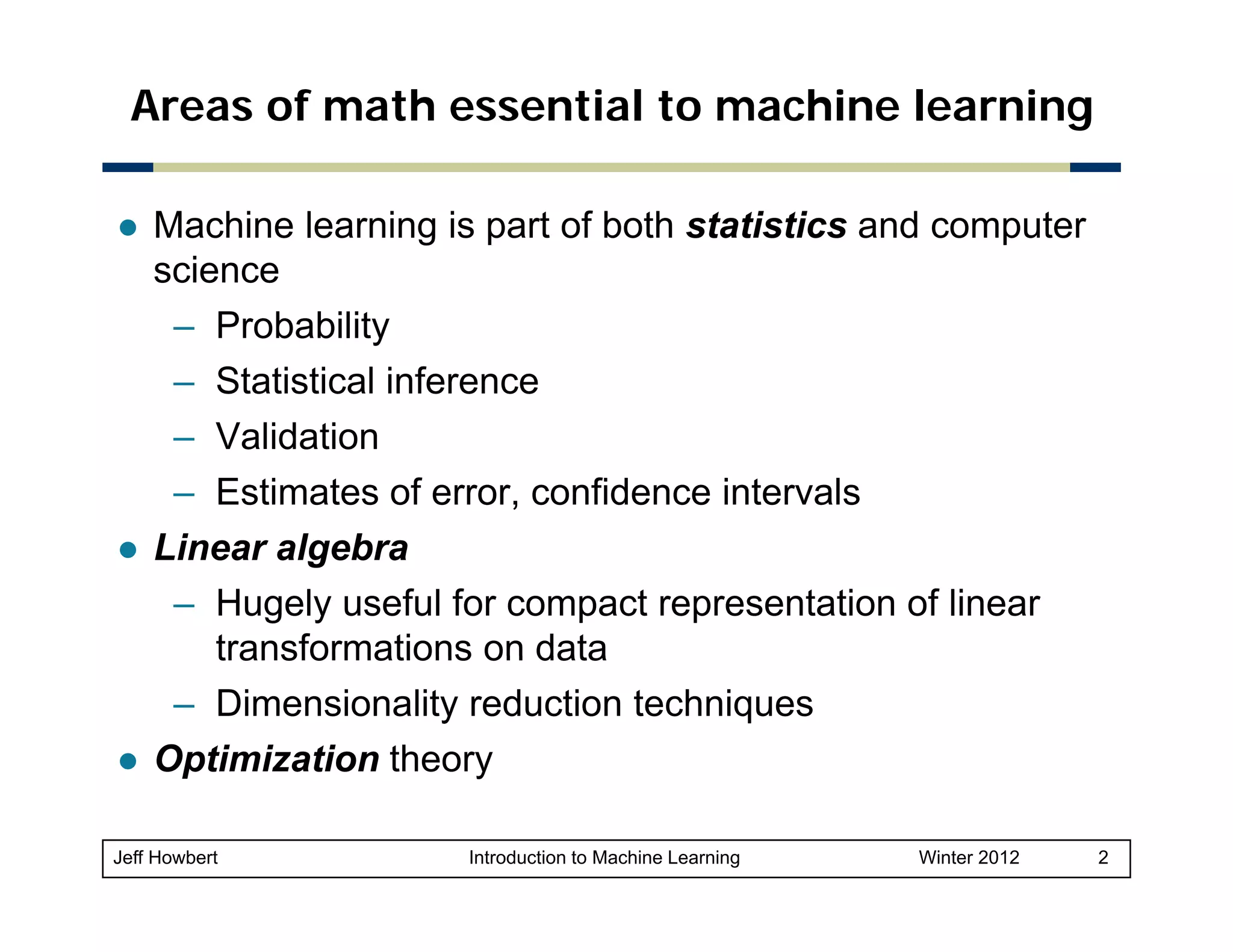
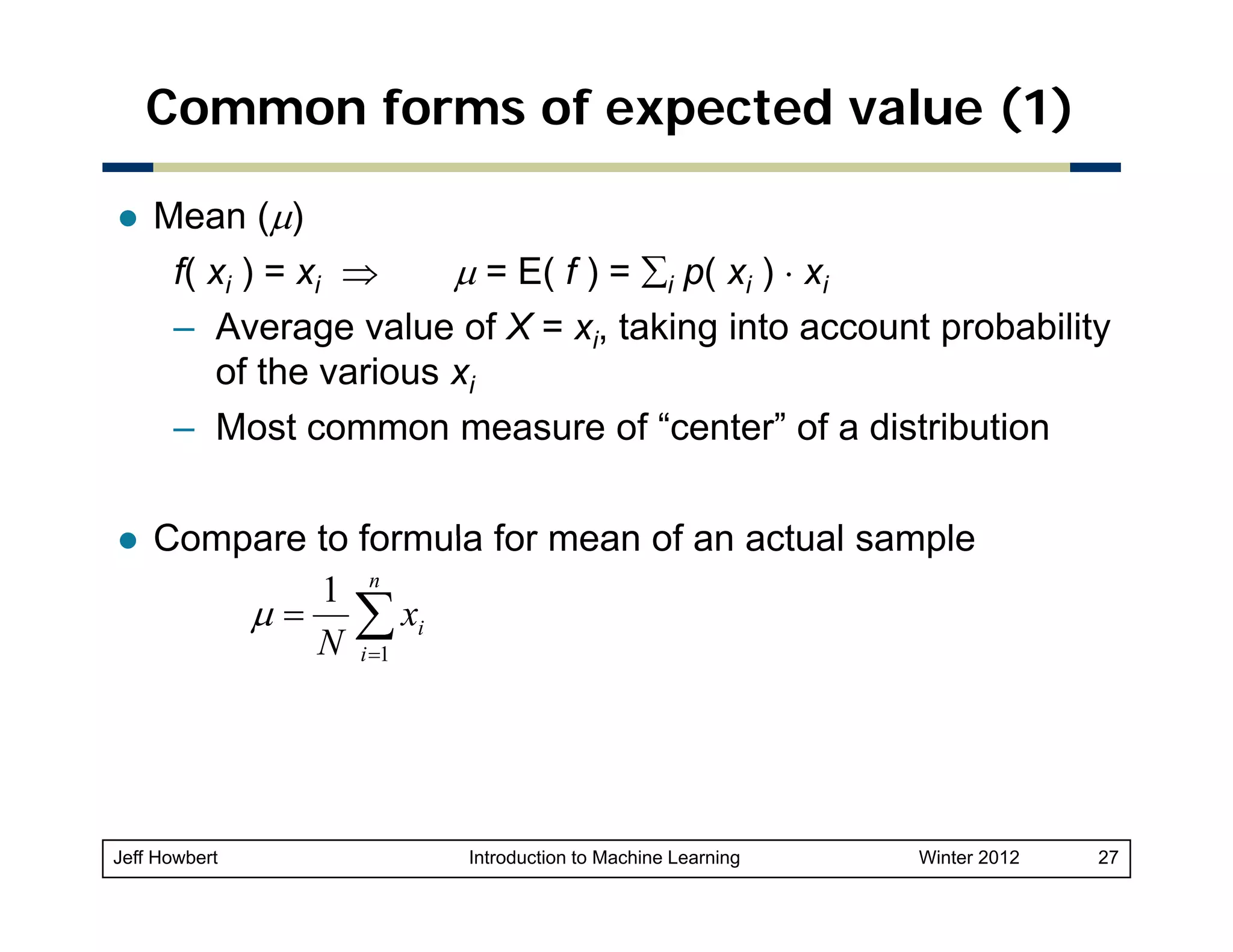
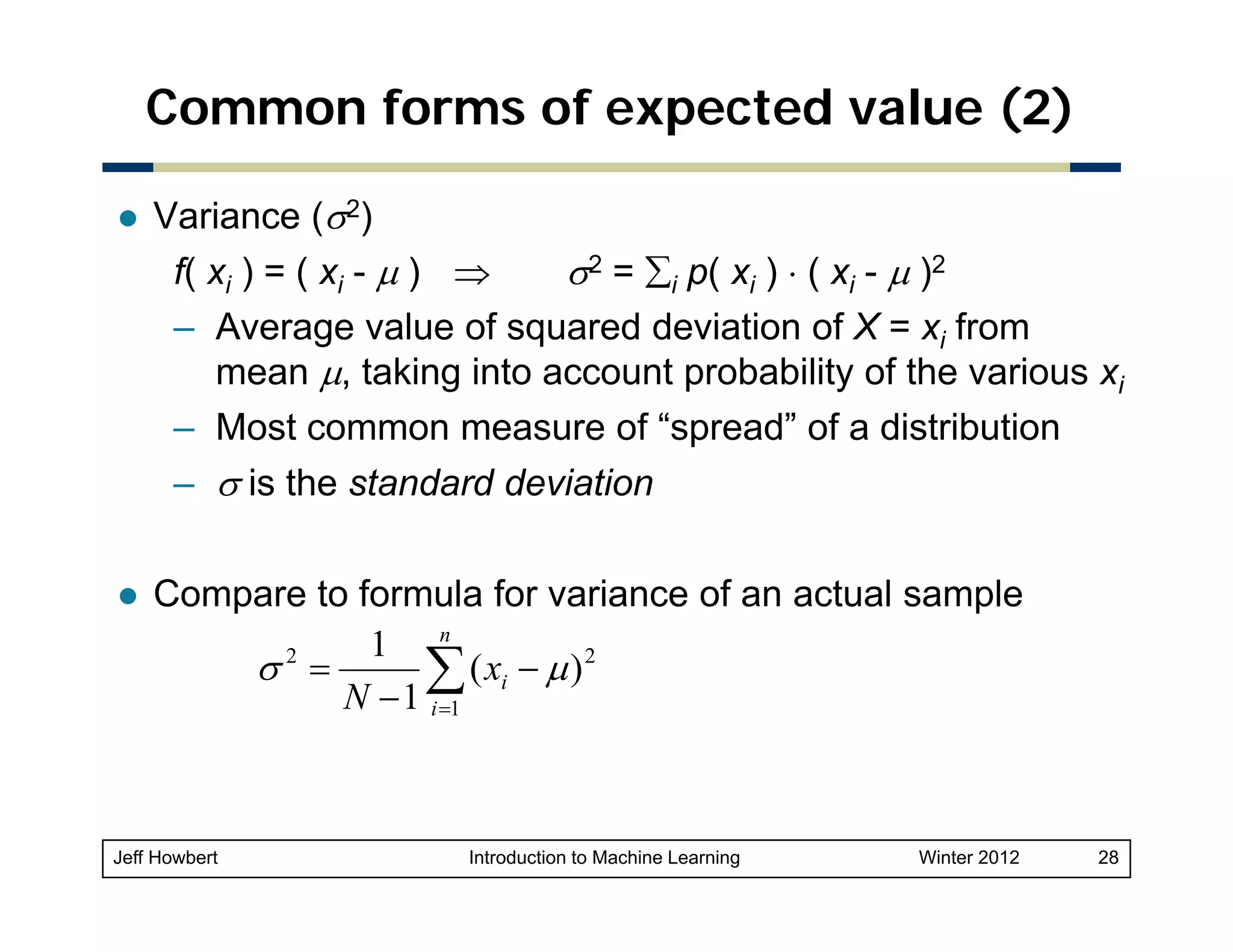
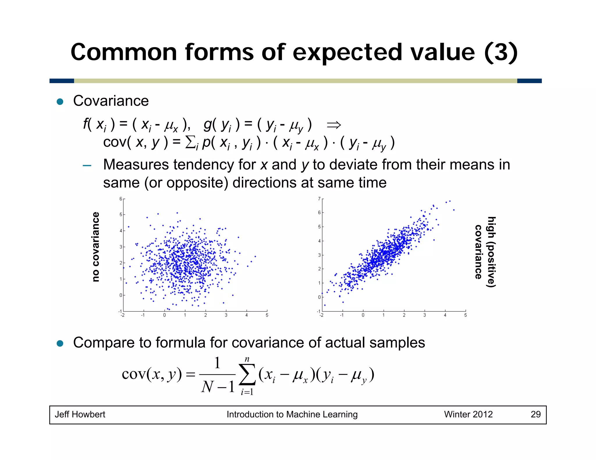
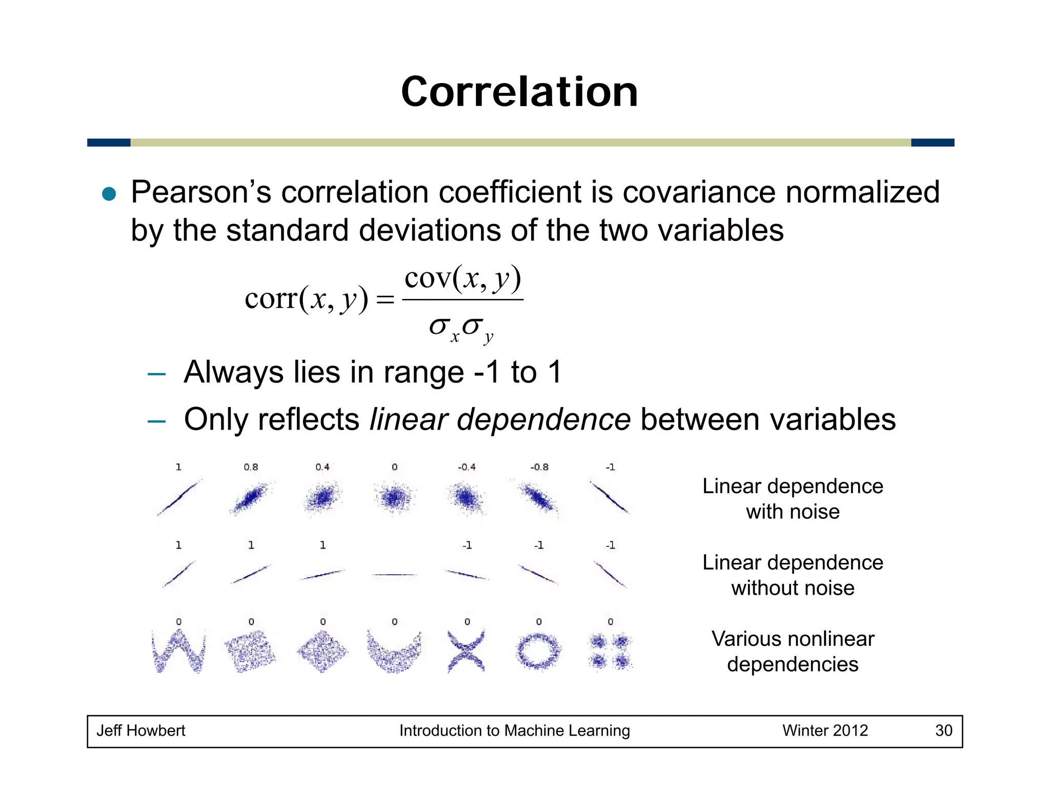
1) Machine learning draws on areas of mathematics including probability, statistical inference, linear algebra, and optimization theory. 2) While there are easy-to-use machine learning packages, understanding the underlying mathematics is important for choosing the right algorithms, making good parameter and validation choices, and interpreting results. 3) Key concepts in probability and statistics that are important for machine learning include random variables, probability distributions, expected value, variance, covariance, and conditional probability. These concepts allow quantification of relationships and uncertainties in data.


![[系列活動] 資料探勘速遊](https://cdn.slidesharecdn.com/ss_thumbnails/0114ycchendmquicktour-170110050658-thumbnail.jpg?width=640&height=640&fit=bounds)


![[DSC 2016] 系列活動:李泳泉 / 星火燎原 - Spark 機器學習初探](https://cdn.slidesharecdn.com/ss_thumbnails/sparkmllib-161026052038-thumbnail.jpg?width=640&height=640&fit=bounds)