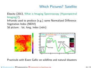
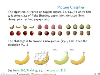
Downloaded 16 times

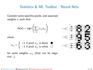
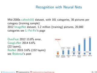
![Statistics & ML Toolbox : Neural Nets
Very popular for pictures...
Picture xi is
• a n×n matrix in {0, 1}n2
for black & white
• a n × n matrix in [0, 1]n2
for grey-scale
• a 3 × n × n array in ([0, 1]3)n2
for color
• a T ×3×n ×n tensor in (([0, 1]3)T )n2
for
video
y here is the label (“8", “9", “6", etc)
Suppose we want to recognize a “6" on a
picture
m(x) =
+1 if x is a “6"
−1 otherwise
@freakonometrics freakonometrics freakonometrics.hypotheses.org 2 / 57](https://image.slidesharecdn.com/lausanne20192-190806161925/85/Lausanne-2019-2-2-320.jpg)


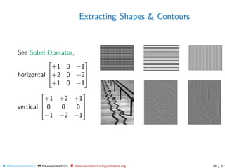
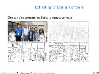
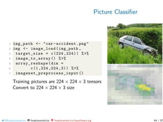
![Picture Classifier
use https://github.com/bnosac/image to extract contours
1 install.packages (" image. LineSegmentDetector ", repos =
"https :// bnosac.github.io/drat ")
2 library(image. LineSegmentDetector )
3 library(imager)
4 img_path <- "../ grey -lausanne.png"
5 im <- load.image(img_path)[,,1,1]
6 linesegments <- image_line_segment_detector (im *255)
7 plot(linesegments)
or
8 library(image. ContourDetector )
9 contourlines <- image_contour_detector (im *255)
10 plot(contourlines)
@freakonometrics freakonometrics freakonometrics.hypotheses.org 28 / 57](https://image.slidesharecdn.com/lausanne20192-190806161925/85/Lausanne-2019-2-28-320.jpg)
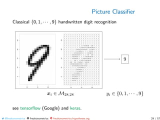
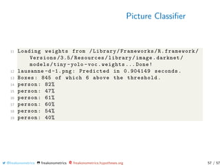
![Picture Classifier
See https://www.tensorflow.org/install
1 library(tensorflow)
2 install_tensorflow (method = "conda ")
3 library(keras)
4 install_keras(method = "conda ")
5 mnist <- dataset_mnist ()
6 idx123 = which(mnist$train$y %in% c(1,2,3))
7 V <- mnist$train$x[idx123 [1:800] , ,]
8 MV = NULL
9 for(i in 1:800) MV=cbind(MV ,as.vector(V[i,,]))
10 MV=t(MV)
11 df=data.frame(y=mnist$train$y[idx123 ][1:800] ,x=MV)
12 reg=glm((y==1)~.,data=df ,family=binomial)
Here xi ∈ R784 (for a small greyscale picture).
@freakonometrics freakonometrics freakonometrics.hypotheses.org 30 / 57](https://image.slidesharecdn.com/lausanne20192-190806161925/85/Lausanne-2019-2-30-320.jpg)
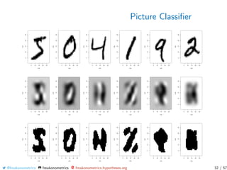
![Picture Classifier
Still with those handwritten digit pictures, from the mnist dataset.
Here {(yi , xi )} with yi = “3” and xi ∈ [0, 1]28×28
One can define a multilinear principal component analysis
see also Tucker decomposition, from Hitchcock (1927, The
expression of a tensor or a polyadic as a sum of products)
We can use those decompositions to derive a simple classifier.
@freakonometrics freakonometrics freakonometrics.hypotheses.org 31 / 57](https://image.slidesharecdn.com/lausanne20192-190806161925/85/Lausanne-2019-2-31-320.jpg)
![Picture Classifier
To reduce dimension use (classical) PCA
1 V <- (mnist$train$x [1:1000 , ,])
2 MV <- NULL
3 for(i in 1:1000) MV <- cbind(MV ,as.vector(V[i,,]))
4 pca <- prcomp(t(MV))
or Multivariate PCA
5 library(rTensor)
6 T <- as.tensor(mnist$train$x [1:1000 , ,])
7 tensor_svd <- hosvd(T)
8 tucker_decomp <- tucker(T, ranks = c(100, 3, 3))
9 T_approx <- ttl(tucker_decomp$Z , tucker_decomp$U , 1:3)
10 pca <- T_approx@data
or directly
11 pca <- mpca(T)
@freakonometrics freakonometrics freakonometrics.hypotheses.org 33 / 57](https://image.slidesharecdn.com/lausanne20192-190806161925/85/Lausanne-2019-2-33-320.jpg)
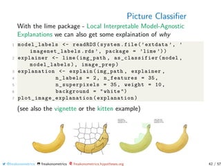
![Picture Classifier
with the (classical) PCA
1 library(factoextra)
2 res.ind <- get_pca_ind(pca)
3 PTS <- res.ind$coord
4 value <- mnist$train$y[idx123 ][1:1000]
Consider a multinomial logistic regression, on the first k
components
5 k <- 10
6 df <- data.frame(y=as.factor(value), x=PTS[,1:k])
7 library(nnet)
8 reg <- multinom(y~.,data=df ,trace=FALSE)
9 df$pred <- predict(reg ,type =" probs ")
@freakonometrics freakonometrics freakonometrics.hypotheses.org 34 / 57](https://image.slidesharecdn.com/lausanne20192-190806161925/85/Lausanne-2019-2-34-320.jpg)
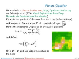
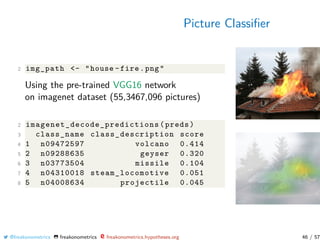
![Picture Classifier
We use here (pre-trained) VGG16 and VGG19 models for Keras,
see Simonyan & Zisserman (2014, Very Deep Convolutional
Networks for Large-Scale Image Recognition)
1 image_prep <- function(x) {
2 arrays <- lapply(x, function(path) {
3 img <- image_load(path , target_size = c(224 ,224))
4 x <- image_to_array(img)
5 x <- array_reshape(x, c(1, dim(x)))
6 x <- imagenet_preprocess_input (x)
7 })
8 do.call(abind ::abind , c(arrays , list(along = 1)))
9 }
10 res <- predict(model , image_prep(img_path))
To create our own model, see Chollet & Allaire (2018, Deep
Learning with R) [github]
@freakonometrics freakonometrics freakonometrics.hypotheses.org 40 / 57](https://image.slidesharecdn.com/lausanne20192-190806161925/85/Lausanne-2019-2-40-320.jpg)
![Picture Classifier
1 imagenet_decode_predictions (res)
2 [[1]]
3 class_name class_description score
4 1 n07753592 banana 0.9929747581
5 2 n03532672 hook 0.0013420789
6 3 n07747607 orange 0.0010816196
7 4 n07749582 lemon 0.0010625814
8 5 n07716906 spaghetti_squash 0.0009176208
with 99.29% chance, the wikipedia picture of a
banana is a banana
@freakonometrics freakonometrics freakonometrics.hypotheses.org 41 / 57](https://image.slidesharecdn.com/lausanne20192-190806161925/85/Lausanne-2019-2-41-320.jpg)

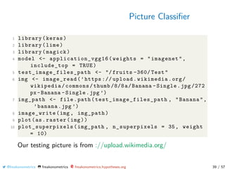
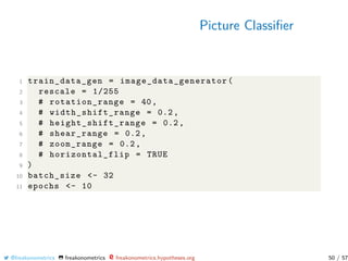
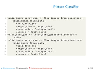
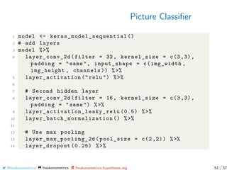
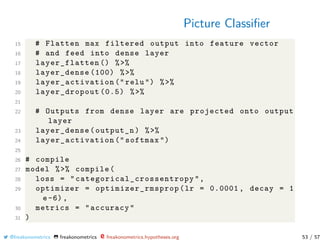
![Picture Classifier
To train our own neural networks, use Chollet & Allaire (2018,
Deep Learning with R) [github]’s code (with keras)
1 channels <- 3
2 img_width <- 20
3 img_height <- 20
4 target_size <- c(img_width , img_height)
5 train_image_files_path <- "../ fruits -360/ Training /"
6 valid_image_files_path <- "../ fruits -360/ Validation /"
7 library(keras)
8 library(lime)
9 library(magick)
10 library(ggplot2)
11 train_samples <- train_image_array_gen$n
12 valid_samples <- valid_image_array_gen$n
@freakonometrics freakonometrics freakonometrics.hypotheses.org 49 / 57](https://image.slidesharecdn.com/lausanne20192-190806161925/85/Lausanne-2019-2-49-320.jpg)


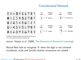
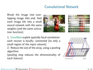
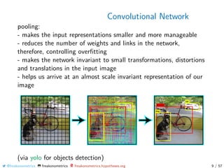
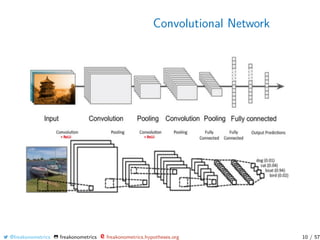
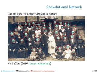
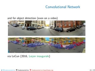
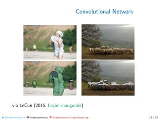
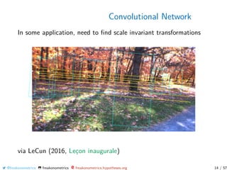
The document discusses various techniques for classifying pictures using neural networks, including convolutional neural networks. It describes how convolutional neural networks can be used to classify images by breaking them into overlapping tiles, applying small neural networks to each tile, and pooling the results. The document also discusses using recurrent neural networks to classify videos by treating them as higher-dimensional tensors.


