Download as PDF, PPTX
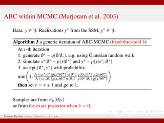
![Nowadays there are several ways to deal with “intractable
likelihoods”, that is models for which an explicit likelihood function
is unavailable.
“Plug-and-play methods”: the only requirements is the ability to
simulate from the data-generating-model.
particle marginal methods (PMMH, PMCMC) based on SMC
filters [Andrieu et al. 2010].
Iterated filtering [Ionides et al. 2011]
approximate Bayesian computation (ABC) [Marin et al. 2012].
In the following I will focus on ABC methods.
Andrieu, Doucet and Holenstein 2010. Particle Markov chain Monte Carlo methods.
JRSS-B.
Ionides, Bhadra, Atchade and King 2011. Iterated filtering. Ann. Stat.
Marin, Pudlo, Robert and Ryder 2012. Approximate Bayesian computational methods.
Stat. Comput.
Umberto Picchini (umberto@maths.lth.se)](https://image.slidesharecdn.com/abcdatacloning-160217215913/85/ABC-with-data-cloning-for-MLE-in-state-space-models-2-320.jpg)
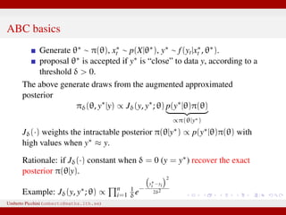
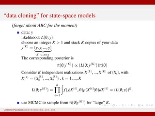
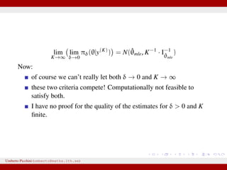
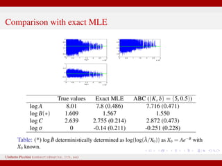
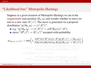
![Asymptotics, K → ∞ (Jacquier et al. 2007; Lele et al. 2007)
K is the # of data “clones”
when K → ∞ we have...
¯θ = sample mean of MCMC draws from π(θ|y(K)) ⇒ ˆθmle
(whatever the prior!)
K× [sample covariance of draws] from π(θ|y(K)) ⇒ I−1
ˆθmle
the
inverse of the Fisher information of the MLE.
¯θ ⇒ N ˆθmle, K−1 · I−1
ˆθmle
1 Jacquier, Johannes, Polson. J. Econometrics (2007)
2 Lele, Dennis, Lutscher. Ecology Letters (2007).
Umberto Picchini (umberto@maths.lth.se)](https://image.slidesharecdn.com/abcdatacloning-160217215913/85/ABC-with-data-cloning-for-MLE-in-state-space-models-15-320.jpg)
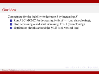
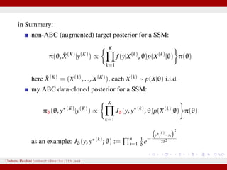
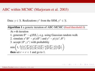
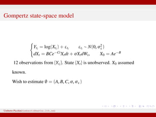
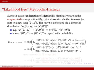
![Stochastic Gompertz model
dXt = BCe−Ct
Xtdt + σXtdWt, X0 = Ae−B
Used in ecology for population growth, e.g. chicken growth data [Donnet,
Foulley, Samson 2010]
0 5 10 15 20 25 30 35 40
0
1
2
3
4
5
6
7
8
9
12 observations from {log Xt}. X0 assumed known.
We wish to estimate θ = (A, B, C, σ)
Exact MLE available as transition densities are known.
Umberto Picchini (umberto@maths.lth.se)](https://image.slidesharecdn.com/abcdatacloning-160217215913/85/ABC-with-data-cloning-for-MLE-in-state-space-models-22-320.jpg)


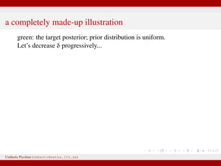
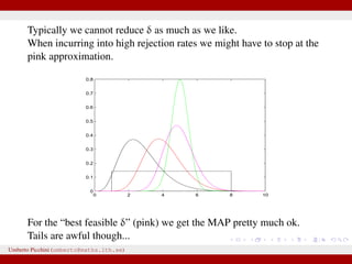
The document discusses maximum likelihood estimation of state-space stochastic differential equation (SDE) models using approximate Bayesian computation (ABC) to handle intractable likelihoods. It focuses on the use of data-cloning methods to improve estimation accuracy by increasing the effective sample size through replicating data. The combination of ABC and data cloning aims to achieve better posterior distribution estimates when traditional methods struggle with low acceptance rates.


![Polymer [ बहुलक ] Chemistry Notes PDF - Irfanullah Mehar - JJ Sir Chemistry.pdf](https://cdn.slidesharecdn.com/ss_thumbnails/polymerchemistrynotespdf-irfanullahmehar-jjsirchemistry-260210172118-3f9b37f7-thumbnail.jpg?width=640&height=640&fit=bounds)


