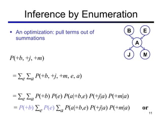
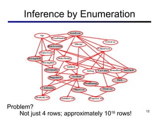
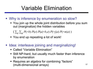
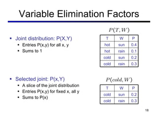
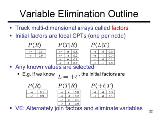
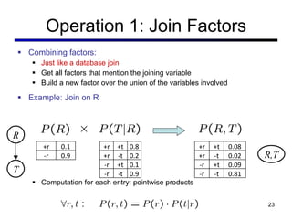
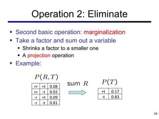
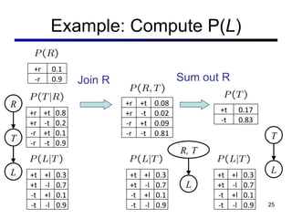
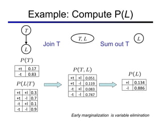
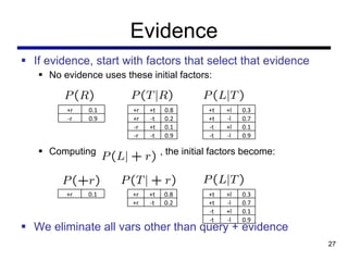
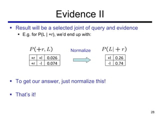
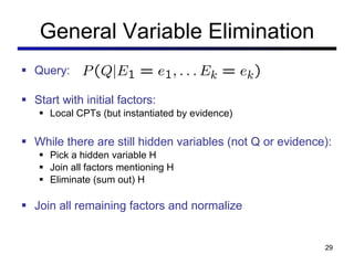
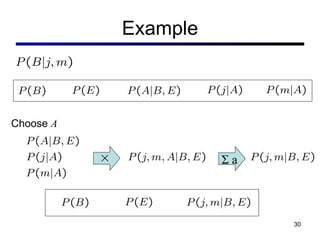
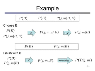
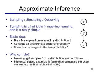
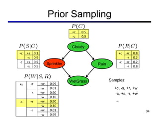
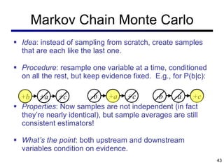
1. CS 221: Artificial Intelligence Lecture 4: Probabilistic Inference Sebastian Thrun and Peter Norvig Slide credit: Dan Klein

4. Probability “ Probability theory is nothing But common sense reduced to calculation.” - Pierre Laplace, 1819 The true logic for this world is the calculus of Probabilities, which takes account of the magnitude of the probability which is, or ought to be, in a reasonable man’s mind.” - James Maxwell, 1850

6. Google Whiteboard

7. Example: Alarm Network B urglary E arthquake A larm J ohn calls M ary calls B P(B) +b 0.001  b 0.999 E P(E) +e 0.002  e 0.998 B E A P(A|B,E) +b +e +a 0.95 +b +e  a 0.05 +b  e +a 0.94 +b  e  a 0.06  b +e +a 0.29  b +e  a 0.71  b  e +a 0.001  b  e  a 0.999 A J P(J|A) +a +j 0.9 +a  j 0.1  a +j 0.05  a  j 0.95 A M P(M|A) +a +m 0.7 +a  m 0.3  a +m 0.01  a  m 0.99

10. Inference by Enumeration P (+ b , + j , + m ) = ∑ e ∑ a P (+ b , + j , + m , e , a ) = ∑ e ∑ a P (+ b ) P ( e ) P ( a |+ b , e ) P (+ j | a ) P (+ m | a ) = B E A J M

12. Inference by Enumeration Not just 4 rows; approximately 10 16 rows! Problem?

13. How can we make inference tractible?

14. Causation and Correlation

15. Causation and Correlation J M A B E B E A J M

16. Causation and Correlation M J E B A B E A J M

25. Example: Compute P( L ) Sum out R T L T R L Join R R, T L +r +t 0.08 +r -t 0.02 -r +t 0.09 -r -t 0.81 +t +l 0.3 +t -l 0.7 -t +l 0.1 -t -l 0.9 +t 0.17 -t 0.83 +t +l 0.3 +t -l 0.7 -t +l 0.1 -t -l 0.9 +r 0.1 -r 0.9 +r +t 0.8 +r -t 0.2 -r +t 0.1 -r -t 0.9 +t +l 0.3 +t -l 0.7 -t +l 0.1 -t -l 0.9

26. Example: Compute P( L ) Join T Sum out T T, L L Early marginalization is variable elimination T L +t 0.17 -t 0.83 +t +l 0.3 +t -l 0.7 -t +l 0.1 -t -l 0.9 +t +l 0.051 +t -l 0.119 -t +l 0.083 -t -l 0.747 +l 0.134 -l 0.886

30. Example Choose A Σ a

31. Example Choose E Finish with B Normalize Σ e

32. Pause for Questions

34. Prior Sampling Cloudy Sprinkler Rain WetGrass Cloudy Sprinkler Rain WetGrass Samples: +c, -s, +r, +w -c, +s, -r, +w … +c 0.5 -c 0.5 +c +s 0.1 -s 0.9 -c +s 0.5 -s 0.5 +c +r 0.8 -r 0.2 -c +r 0.2 -r 0.8 +s +r +w 0.99 -w 0.01 -r +w 0.90 -w 0.10 -s +r +w 0.90 -w 0.10 -r +w 0.01 -w 0.99

40. Likelihood Weighting Samples: +c, +s, +r, +w … Cloudy Sprinkler Rain WetGrass Cloudy Sprinkler Rain WetGrass 0.099 +c 0.5 -c 0.5 +c +s 0.1 -s 0.9 -c +s 0.5 -s 0.5 +c +r 0.8 -r 0.2 -c +r 0.2 -r 0.8 +s +r +w 0.99 -w 0.01 -r +w 0.90 -w 0.10 -s +r +w 0.90 -w 0.10 -r +w 0.01 -w 0.99

46. Monty Hall on Monty Hall Problem

47. Monty Hall on Monty Hall Problem