The document discusses production with two variable inputs of capital and labor. It explains that firms can produce different levels of output by varying the amounts of capital and labor used. Isoquants show all the combinations of inputs that produce the same level of output. The isoquant curves are downward sloping, showing diminishing marginal rate of technical substitution between the two inputs. Holding one input constant and increasing the other results in diminishing marginal returns. The isoquant curves are convex due to the law of diminishing marginal returns. Different types of isoquants represent perfect substitutes, perfect complements, and fixed proportions production functions. The document also discusses minimizing costs using isoquants and isocost curves to determine the optimal input

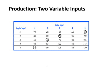
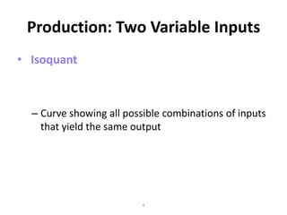
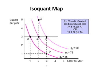
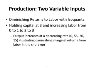
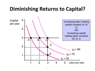
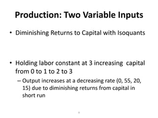
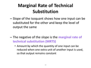
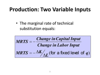
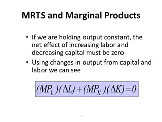
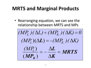
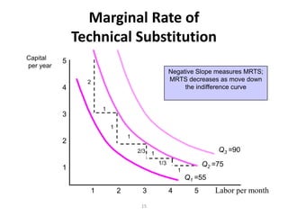
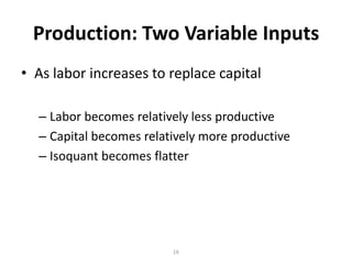
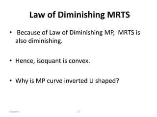
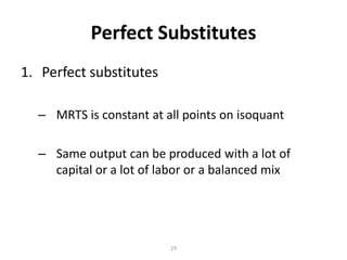
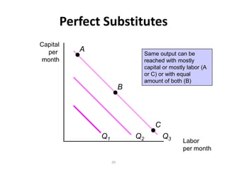
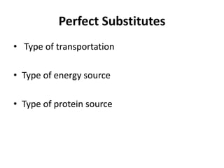
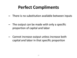
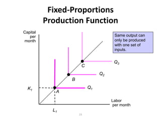
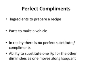
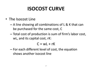
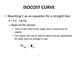
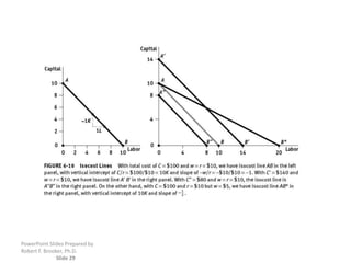
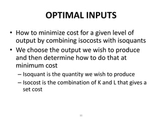
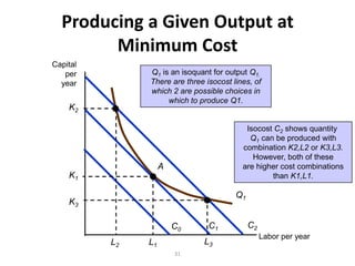
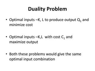
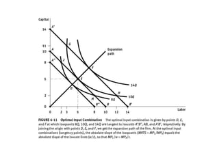
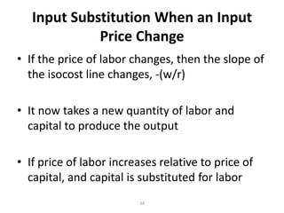
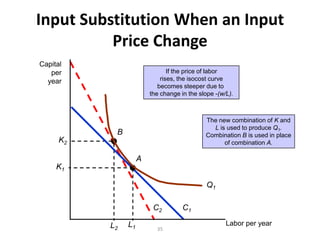
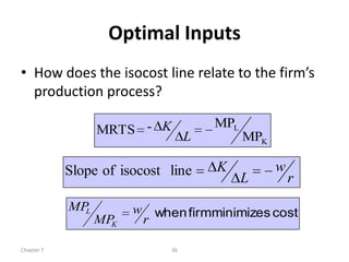
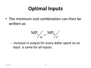
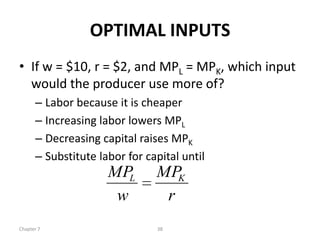
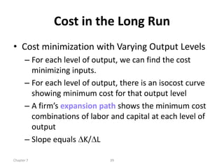
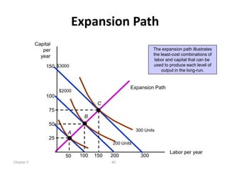
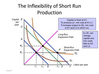
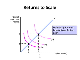
1. PRODUCTION WITH TWO INPUTS
1

2. Production: Two Variable Inputs
• Firm can produce output by combining
different amounts of labor and capital
• In the long run, capital and labor are both
variable
2

3. Production: Two Variable Inputs
3

4. Production: Two Variable Inputs
• Isoquant
– Curve showing all possible combinations of inputs
that yield the same output
4

5. Isoquant Map
Capital 5 E
Ex: 55 units of output
per year can be produced with
3K & 1L (pt. A)
4 OR
1K & 3L (pt. D)
3
A B C
2
q3 = 90
D q2 = 75
1
q1 = 55
1 2 3 4 5 Labor per year
5

6. Production: Two Variable Inputs
• Diminishing Returns to Labor with Isoquants
• Holding capital at 3 and increasing labor from
0 to 1 to 2 to 3
– Output increases at a decreasing rate (0, 55, 20,
15) illustrating diminishing marginal returns from
labor in the short run
6

7. Diminishing Returns to Capital?
Capital 5 Increasing labor holding
per year capital constant (A, B,
C)
4 OR
Increasing capital
holding labor constant
3 (E, D, C
A B C
D
2
q3 = 90
1 E q2 = 75
q1 = 55
1 2 3 4 5 Labor per year
7

8. Production: Two Variable Inputs
• Diminishing Returns to Capital with Isoquants
• Holding labor constant at 3 increasing capital
from 0 to 1 to 2 to 3
– Output increases at a decreasing rate (0, 55, 20,
15) due to diminishing returns from capital in
short run
8

9. ISOQUANTS
• Why are isoquant curve downward sloping?

10. Marginal Rate of Technical
Substitution
– Slope of the isoquant shows how one input can be
substituted for the other and keep the level of
output the same
– The negative of the slope is the marginal rate of
technical substitution (MRTS)
• Amount by which the quantity of one input can be
reduced when one extra unit of another input is used,
so that output remains constant
10

11. Production: Two Variable Inputs
• The marginal rate of technical
substitution equals:
Change in Capital Input
MRTS
Change in Labor Input
MRTS K (for a fixed level of q )
L
11

12. MRTS and Marginal Products
• If we are holding output constant, the
net effect of increasing labor and
decreasing capital must be zero
• Using changes in output from capital and
labor we can see
(MPL )( L) (MPK )( K) 0
12

13. MRTS and Marginal Products
• Rearranging equation, we can see the
relationship between MRTS and MPs
(MP )( L) (MP )( K) 0
L K
(MP )( L) - (MP )( K)
L K
(MP )
L L
MRTS
( MPK ) K
13

14. ISOQUANT
• Why is isoquant convex to the origin?

15. Marginal Rate of
Technical Substitution
Capital 5
per year
Negative Slope measures MRTS;
2 MRTS decreases as move down
4 the indifference curve
1
3
1
1
2
2/3 1
Q3 =90
1/3 Q2 =75
1 1
Q1 =55
1 2 3 4 5 Labor per month
15

16. Production: Two Variable Inputs
• As labor increases to replace capital
– Labor becomes relatively less productive
– Capital becomes relatively more productive
– Isoquant becomes flatter
16

17. Law of Diminishing MRTS
• Because of Law of Diminishing MP, MRTS is
also diminishing.
• Hence, isoquant is convex.
• Why is MP curve inverted U shaped?
Chapter 6 17

18. SPECIAL ISOQUANTS
18

19. Perfect Substitutes
1. Perfect substitutes
– MRTS is constant at all points on isoquant
– Same output can be produced with a lot of
capital or a lot of labor or a balanced mix
19

20. Perfect Substitutes
Capital
per A
Same output can be
month reached with mostly
capital or mostly labor (A
or C) or with equal
amount of both (B)
B
C
Q1 Q2 Q3
Labor
per month
20

21. Perfect Substitutes
• Type of transportation
• Type of energy source
• Type of protein source

22. Perfect Compliments
– There is no substitution available between inputs
– The output can be made with only a specific
proportion of capital and labor
– Cannot increase output unless increase both
capital and labor in that specific proportion
22

23. Fixed-Proportions
Production Function
Capital
per Same output can
month only be produced
with one set of
inputs.
Q3
C
Q2
B
K1 Q1
A
Labor
per month
L1
23

24. Perfect Compliments
• Ingredients to prepare a recipe
• Parts to make a vehicle
• In reality there is no perfect substitute /
compliments
• Ability to substitute one i/p for the other
diminishes as one moves along Isoquant

25. MINIMIZING COST
Chapter 6 25

26. Cost Minimizing Input Choice
• How do we put all this together to select inputs to produce
a given output at minimum cost?
• Assumptions
– Two Inputs: Labor (L) and capital (K)
– Price of labor: wage rate (w)
– The price of capital
26

27. ISOCOST CURVE
• The Isocost Line
– A line showing all combinations of L & K that can
be purchased for the same cost, C
– Total cost of production is sum of firm’s labor cost,
wL, and its capital cost, rK:
C = wL + rK
– For each different level of cost, the equation
shows another isocost line
27

28. ISOCOST CURVE
• Rewriting C as an equation for a straight line:
K = C/r - (w/r)L
– Slope of the isocost:
• -(w/r) is the ratio of the wage rate to rental cost of
capital.
• This shows the rate at which capital can be substituted
for labor with no change in cost
K w
L r
28

29. PowerPoint Slides Prepared by
Robert F. Brooker, Ph.D.
Slide 29

30. OPTIMAL INPUTS
• How to minimize cost for a given level of
output by combining isocosts with isoquants
• We choose the output we wish to produce
and then determine how to do that at
minimum cost
– Isoquant is the quantity we wish to produce
– Isocost is the combination of K and L that gives a
set cost
30

31. Producing a Given Output at
Minimum Cost
Capital
per Q1 is an isoquant for output Q1.
year There are three isocost lines, of
which 2 are possible choices in
which to produce Q1.
K2
Isocost C2 shows quantity
Q1 can be produced with
combination K2,L2 or K3,L3.
However, both of these
A are higher cost combinations
K1 than K1,L1.
Q1
K3
C0 C1 C2
Labor per year
L2 L1 L3
31

32. Duality Problem
• Optimal inputs –K, L to produce output Q1 and
minimize cost
• Optimal inputs –K,L with cost C1 and
maximize output
• Both these problems would give the same
optimal input combination

34. Input Substitution When an Input
Price Change
• If the price of labor changes, then the slope of
the isocost line changes, -(w/r)
• It now takes a new quantity of labor and
capital to produce the output
• If price of labor increases relative to price of
capital, and capital is substituted for labor
34

35. Input Substitution When an Input
Price Change
Capital
per If the price of labor
year rises, the isocost curve
becomes steeper due to
the change in the slope -(w/L).
The new combination of K and
L is used to produce Q1.
B Combination B is used in place
K2 of combination A.
A
K1
Q1
C2 C1
L2 L1 Labor per year
35

36. Optimal Inputs
• How does the isocost line relate to the firm’s
production process?
MRTS - K MPL
L MPK
Slope of isocost line K w
L r
MPL w when firmminimizes cost
MPK r
Chapter 7 36

37. Optimal Inputs
• The minimum cost combination can then be
written as:
MPL MPK
w r
– Increase in output for every dollar spent on an
input is same for all inputs.
Chapter 7 37

38. OPTIMAL INPUTS
• If w = $10, r = $2, and MPL = MPK, which input
would the producer use more of?
– Labor because it is cheaper
– Increasing labor lowers MPL
– Decreasing capital raises MPK
– Substitute labor for capital until
MPL MPK
w r
Chapter 7 38

39. Cost in the Long Run
• Cost minimization with Varying Output Levels
– For each level of output, we can find the cost
minimizing inputs.
– For each level of output, there is an isocost curve
showing minimum cost for that output level
– A firm’s expansion path shows the minimum cost
combinations of labor and capital at each level of
output
– Slope equals K/ L
Chapter 7 39

40. Expansion Path
Capital
per The expansion path illustrates
year the least-cost combinations of
labor and capital that can be
150 $3000 used to produce each level of
output in the long-run.
Expansion Path
$2000
100
C
75
B
50
300 Units
A
25
200 Units
Labor per year
50 100 150 200 300
Chapter 7 40

41. Expansion Path
• It shows optimal input combinations to minimize
cost to produce different levels of output
• It shows the minimum cost to produce different
levels of output
• It shows the maximum amount of output that can
be produced for different levels of expenditure.

42. A Firm’s Long Run Total Cost Curve
Cost/
Year
Long Run Total Cost
F
3000
E
2000
D
1000
Output, Units/yr
100 200 300
Chapter 7 42

44. Long Run Versus Short Run Cost
Curves
• In the short run, some costs are fixed
• In the long run, firm can change anything
including plant size
– Can produce at a lower average cost in long run
than in short run
– Capital and labor are both flexible
• We can show this by holding capital fixed in
the short run and flexible in long run
Chapter 7 44

45. The Inflexibility of Short Run
Production
Capital E Capital is fixed at K1.
per To produce q1, min cost at K1,L1.
year If increase output to Q2, min cost
C is K1 and L3 in short run.
In LR, can
Long-Run
change
Expansion Path
A capital and
min costs
falls to K2
K2 and L2.
Short-Run
P Expansion Path
K1 Q2
Q1
Labor per year
L1 L2 B L3 D F
Chapter 7 45

46. RETURNS TO SCALE
46

47. BIG CITIES
• Metropolis twice the size of one, number of
gas stations, length of pipelines, infrastructure
decreases by 15%
• Why?
47

48. Narayan
Hridalaya
• Provide health care at full price
To patients from well to do background
• These patients subsidize `poor’ patients
• Run at a profit of 7.7%
• Why is Narayan Hridalaya able to do this?
48

49. Narayan
Hridalaya
• Number of Beds, 2001: 225
• Current No. of Beds across India: 30,000
• How does number of beds play a role in
profits?
49

50. Returns to Scale
• Rate at which output increases as inputs are
increased proportionately
– Increasing returns to scale
– Constant returns to scale
– Decreasing returns to scale
50

51. Returns to Scale
• Increasing returns to scale: output more than
doubles when all inputs are doubled
– What happens to the isoquants?
51

52. Increasing Returns to Scale
Capital
(machine The isoquants
hours) A
move closer
together
4
30
2 20
10
Labor (hours)
5 10
52

53. Returns to Scale
• Constant returns to scale: output doubles
when all inputs are doubled
– Size does not affect productivity
– May have a large number of producers
– Isoquants are equidistant apart
53

54. Returns to Scale
Capital
(machine
A
hours)
6
30
4 Constant Returns:
Isoquants are
2 equally spaced
0
2
10
Labor (hours)
5 10 15
54

55. Returns to Scale
• Decreasing returns to scale: output less than
doubles when all inputs are doubled
– Decreasing efficiency with large size
– Reduction of entrepreneurial abilities
– Isoquants become farther apart
55

56. Returns to Scale
Capital
(machine A
hours)
Decreasing Returns:
Isoquants get further
4 apart
30
2
20
10
5 10 Labor (hours)
56