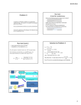
04-09-2012


       Understanding Equivalent calculations                                                                                                                   Understanding Equivalent calculations
                                                  n (n + 1)
                    Test Statistic U = n1n2 + 1 1           − R1
                                                      2
                    = # of ( X i , Y j ) pairs where X i < Y j
                                                                                                                                                       The p-value and hence the conclusion would be the same
                                                          n1n2                         n1n2 (n1 + n2 + 1)                                              irrespective of what form of the test statistic is used, i.e.
                    Under H 0 , µU =                           ,          σU =
                                                           2                                  12                                                                                       R1 or R2                         ɶ
                                                                                                                                                                                                                or U or U
                                  U-µ U
                    and                      has N(0,1) distribution                                                                                   But need to be careful on (a) left or right tailed, depending on the
                                   σU
                                                                                n ( n + 1)
                                                                                                                                                       form (b) Mean to be subtracted (S.E would be the same)
         (n1 + n2 )( n1 + n2 + 1)                                   ɶ
                                                                   U = n1n2 + 2 2            − R2
R1 + R2 =                                                                             2
                      2
                       n ( n + n + 1)
                                                                   = # of ( X i , Y j ) pairs where X i > Y j
Under H 0 : E ( R1 ) = 1 1 2
                              2                                         ɶ
                                                                   U + U = n1n2
                                                                      ɶ nn    nn
                                                                   ⇒ U − 1 2 = 1 2 −U
                                                                         2     2


               Numerical illustration: small sample                                                                                                                   14-34 in Aczel -Sounderpandyan
                 Q. Do Model B planes fly faster? (modified ex14.4)
                 Travel time in two models of copter-planes :
                                                                                                                                                           Test if the (average) current ratio for the 3 industries are the same.
                 Model A: 35                    38         40 43                  n1 = 4
                 Model B: 27                    29          36                n2 = 3
                 R1 = 3 + 5 + 6 + 7 = 21                           R2 = 1 + 2 + 4 = 7
                         4×5                                                                                                                                                                                                             mean sd
                U = 12 +     − 21 = 1 Easier to note this directly from pairs!
                           2
                 p-value=P(U ≤ 1) = 0.0571 (Table 9 in P798)
                                                                                                                                                       A              1.38 1.55                 1.9       2     1.22 2.11 1.98 1.61      1.719 0.324
         Note that the distribution of U is symmetric (about…?) under the null hypothesis
                                                                                           Let the rank of X obs. be r1 ,… rn1 . R1 = r1 + … + rn1
                                                                                                                                        n1 ( n1 − 1)
                                                                                                                                                       B              2.33         2.5          2.79 3.01 1.99 2.45                      2.512 0.356
    Can you see why U = No. of (X i , Y j ) pairs with X i < Y j                           U = (n1 + n2 − r1 ) + … (n1 + n2 − rn1 ) −
               n1 (n1 + 1)                                                                                                                    2
    = n1n2 +               − R1                                                                                      n1 ( n1 − 1)
                    2                                                                      = n1 ( n1 + n2 ) − R1 −
                                                                                                                           2                           C              1.06 1.37 1.09 1.65 1.44 1.11                                      1.287 0.238
                                                                                                      n1 (n1 + 1)
                                                                                           = n1n2 +               − R1
                                                                                                           2


                                        Kruskal-Wallis Test                                                                                                       Solving 14-34 using Kruskal-Wallis
                                                                                                                                                           Industry    current ratio     rank

         • For comparing means of more than 2                                                                                                                A
                                                                                                                                                             A
                                                                                                                                                                         1.38
                                                                                                                                                                         1.55
                                                                                                                                                                                          6
                                                                                                                                                                                          8
           populations – alternative to ANOVA                                                                                                                A            1.9            11
                                                                                                                                                             A             2             14                        ranksum sample size R^2/n
         • Use if data is ordinal or the assumptions of                                                                                                      A           1.22             4           A                79       8        780.125
           ANOVA are violated                                                                                                                                A
                                                                                                                                                             A
                                                                                                                                                                         2.11
                                                                                                                                                                         1.98
                                                                                                                                                                                         15
                                                                                                                                                                                         12           B               103         6        1768.167
         • Pull all observations and rank them                                                                                                               A           1.61             9
                                                                                                                                                             B           2.33            16           C               28          6        130.6667
         • Compute total of the ranks of observations                                                                                                        B            2.5            18
                                                                                                                                                             B           2.79            19           total           210        20       2678.958
           coming from 1st, 2nd ,3rd… populations                                                                                                            B           3.01            20
                                                                                                                                                             B           1.99            13
         • Null distribution is Chi-square with k-1 d.f                                                                                                      B           2.45            17                   12 × 2678.96
                                                                                                                                                             C           1.06             1           T.S. is                − 3 × 21 = 13.54
                                                  12        R                 2                                                                              C           1.37             5                      20 × 21
                                  T.S. is
                                                n(n + 1 )
                                                          ∑ n − 3(n + 1 )    i                                                                               C
                                                                                                                                                             C
                                                                                                                                                                         1.09
                                                                                                                                                                         1.65
                                                                                                                                                                                          2
                                                                                                                                                                                         10           p − value = P(χ 2 df > 13.54) = 0.001
                                                                                                                                                                                                                       2
                                                             i
                                                                                                                                                             C           1.44             7
                                                                                                                                                             C           1.11             3


                                                                                                                                                                                                                                                        1
04-09-2012


                                                                                                              Run test:
                                   Problem 3
                                                                                                       A test for randomness
                                                                                        • Which of the following sequences appear to be ‘random’?
                                                                                            – HTHTHTHTHTHTHTHTHTHTHTHTHTHTHTHT
                                                                                            – HHHHHHHHHHHHHHTTTTTTTTTTTTTTTTTT
             A sequence of small glass sculptures was inspected for                         – HHHHHHHHHHHTTTTTTTTTTTHHHHHHHHH
             shipping damage. The sequence of acceptable and damaged                    •   NONE! How to determine objectively or statistically?
             pieces was as follows:                                                     •   Calculate the no. of runs
                                                                                        •   A run is a sequence of identical symbols/events
             D,A,A,A,D,D,D,D,D,A,A,D,D,A,A,A,A,D,A,A,D,D,D,D,D                          •   Too many (or few) runs indicate lack of randomness
                                                                                            – HTHT HTHT HTHT HTHT HTHT HTHT HTHT HT
                                                                                            – HHHHHHHHHHHHHHTTTTTTTTTTTTTTTTTT
             Test for the randomness of the damage to the shipment using                    – HHHHHHHHHHHTTTTTTTTTTTHHHHHHHHH
             the 0.05 significance level.


                          Run test (cont.)                                                           Solution to Problem 3
    • How to determine too many or too few?
    • Acceptable no. of runs depend on n1, n2                                           nA = 11, nD = 14,
                                                                                             2 × 11× 14
  If H 0 (the sequence is 'randomly' mixed) is true,
                                                       r-µr
                                                              has approximately         µr =            + 1 = 13.32,
                                                       σr                                     11 + 14
  N(0,1) distribution, provided either n1or n 2 moderately large ( ≥ 10).                      2 × 11×14(2 ×11× 14 − 25)
  Small sample distributions are avaliable (Table 8 page 796-797).
                                                                                        σr =                                 = 2.41
                                                                                                        25 2 × 24
                                                                                        Atα = 0.05, the C.R. is | Z | > 1.96.
                       2n1n2                2n1n2 (2n1n2 − n1 − n2 )
                                                                                                                                  9 - 13.32
            µr =              +1    σr =                                                The observed r = 9, and value of the T.S. is        = −1.79.
                      n1 + n2               (n1 + n2 )2 (n1 + n2 − 1)                                                                2.41
                                                                                        So at 5% level we conclude that damages occur randomly


Data summarization           Expected Value
 And presentation           in decision making
                              Decision trees Discrete: General, Binomial, Poisson


    Probability             Random variable
                           And its Distribution
                                              Continuous: General, Normal,Exponential
                                                        T, Chi-square, F

    Confidence interval/
     Testing hypothesis                                      Sampling
                                                       Sampling distribution of
                  π                                             X,   p, S 2
  1 or 2
                  µ
 sample
                  σ
                                            Goodness of Fit
            ANOVA                                                                 NP
  Test for indep/homogeneity


                                                                                                                                                            2

Session 20

  • 1.
    04-09-2012 Understanding Equivalent calculations Understanding Equivalent calculations n (n + 1) Test Statistic U = n1n2 + 1 1 − R1 2 = # of ( X i , Y j ) pairs where X i < Y j The p-value and hence the conclusion would be the same n1n2 n1n2 (n1 + n2 + 1) irrespective of what form of the test statistic is used, i.e. Under H 0 , µU = , σU = 2 12 R1 or R2 ɶ or U or U U-µ U and has N(0,1) distribution But need to be careful on (a) left or right tailed, depending on the σU n ( n + 1) form (b) Mean to be subtracted (S.E would be the same) (n1 + n2 )( n1 + n2 + 1) ɶ U = n1n2 + 2 2 − R2 R1 + R2 = 2 2 n ( n + n + 1) = # of ( X i , Y j ) pairs where X i > Y j Under H 0 : E ( R1 ) = 1 1 2 2 ɶ U + U = n1n2 ɶ nn nn ⇒ U − 1 2 = 1 2 −U 2 2 Numerical illustration: small sample 14-34 in Aczel -Sounderpandyan Q. Do Model B planes fly faster? (modified ex14.4) Travel time in two models of copter-planes : Test if the (average) current ratio for the 3 industries are the same. Model A: 35 38 40 43 n1 = 4 Model B: 27 29 36 n2 = 3 R1 = 3 + 5 + 6 + 7 = 21 R2 = 1 + 2 + 4 = 7 4×5 mean sd U = 12 + − 21 = 1 Easier to note this directly from pairs! 2 p-value=P(U ≤ 1) = 0.0571 (Table 9 in P798) A 1.38 1.55 1.9 2 1.22 2.11 1.98 1.61 1.719 0.324 Note that the distribution of U is symmetric (about…?) under the null hypothesis Let the rank of X obs. be r1 ,… rn1 . R1 = r1 + … + rn1 n1 ( n1 − 1) B 2.33 2.5 2.79 3.01 1.99 2.45 2.512 0.356 Can you see why U = No. of (X i , Y j ) pairs with X i < Y j U = (n1 + n2 − r1 ) + … (n1 + n2 − rn1 ) − n1 (n1 + 1) 2 = n1n2 + − R1 n1 ( n1 − 1) 2 = n1 ( n1 + n2 ) − R1 − 2 C 1.06 1.37 1.09 1.65 1.44 1.11 1.287 0.238 n1 (n1 + 1) = n1n2 + − R1 2 Kruskal-Wallis Test Solving 14-34 using Kruskal-Wallis Industry current ratio rank • For comparing means of more than 2 A A 1.38 1.55 6 8 populations – alternative to ANOVA A 1.9 11 A 2 14 ranksum sample size R^2/n • Use if data is ordinal or the assumptions of A 1.22 4 A 79 8 780.125 ANOVA are violated A A 2.11 1.98 15 12 B 103 6 1768.167 • Pull all observations and rank them A 1.61 9 B 2.33 16 C 28 6 130.6667 • Compute total of the ranks of observations B 2.5 18 B 2.79 19 total 210 20 2678.958 coming from 1st, 2nd ,3rd… populations B 3.01 20 B 1.99 13 • Null distribution is Chi-square with k-1 d.f B 2.45 17 12 × 2678.96 C 1.06 1 T.S. is − 3 × 21 = 13.54 12 R 2 C 1.37 5 20 × 21 T.S. is n(n + 1 ) ∑ n − 3(n + 1 ) i C C 1.09 1.65 2 10 p − value = P(χ 2 df > 13.54) = 0.001 2 i C 1.44 7 C 1.11 3 1
  • 2.
    04-09-2012 Run test: Problem 3 A test for randomness • Which of the following sequences appear to be ‘random’? – HTHTHTHTHTHTHTHTHTHTHTHTHTHTHTHT – HHHHHHHHHHHHHHTTTTTTTTTTTTTTTTTT A sequence of small glass sculptures was inspected for – HHHHHHHHHHHTTTTTTTTTTTHHHHHHHHH shipping damage. The sequence of acceptable and damaged • NONE! How to determine objectively or statistically? pieces was as follows: • Calculate the no. of runs • A run is a sequence of identical symbols/events D,A,A,A,D,D,D,D,D,A,A,D,D,A,A,A,A,D,A,A,D,D,D,D,D • Too many (or few) runs indicate lack of randomness – HTHT HTHT HTHT HTHT HTHT HTHT HTHT HT – HHHHHHHHHHHHHHTTTTTTTTTTTTTTTTTT Test for the randomness of the damage to the shipment using – HHHHHHHHHHHTTTTTTTTTTTHHHHHHHHH the 0.05 significance level. Run test (cont.) Solution to Problem 3 • How to determine too many or too few? • Acceptable no. of runs depend on n1, n2 nA = 11, nD = 14, 2 × 11× 14 If H 0 (the sequence is 'randomly' mixed) is true, r-µr has approximately µr = + 1 = 13.32, σr 11 + 14 N(0,1) distribution, provided either n1or n 2 moderately large ( ≥ 10). 2 × 11×14(2 ×11× 14 − 25) Small sample distributions are avaliable (Table 8 page 796-797). σr = = 2.41 25 2 × 24 Atα = 0.05, the C.R. is | Z | > 1.96. 2n1n2 2n1n2 (2n1n2 − n1 − n2 ) 9 - 13.32 µr = +1 σr = The observed r = 9, and value of the T.S. is = −1.79. n1 + n2 (n1 + n2 )2 (n1 + n2 − 1) 2.41 So at 5% level we conclude that damages occur randomly Data summarization Expected Value And presentation in decision making Decision trees Discrete: General, Binomial, Poisson Probability Random variable And its Distribution Continuous: General, Normal,Exponential T, Chi-square, F Confidence interval/ Testing hypothesis Sampling Sampling distribution of π X, p, S 2 1 or 2 µ sample σ Goodness of Fit ANOVA NP Test for indep/homogeneity 2