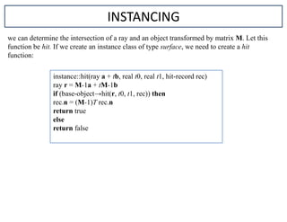
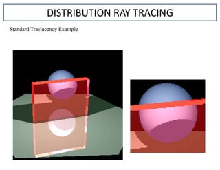
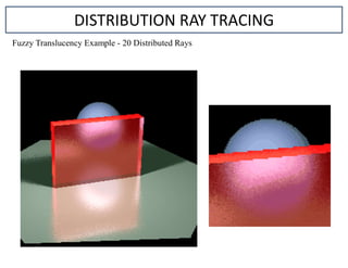
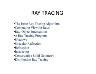
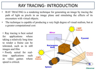
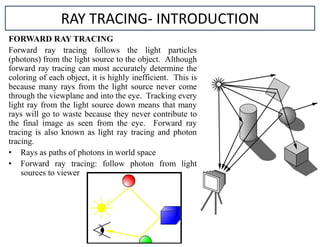
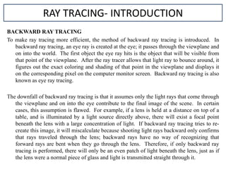
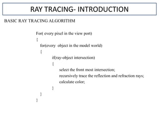
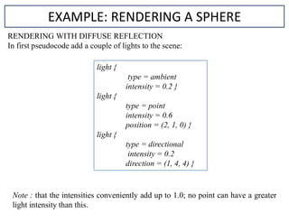
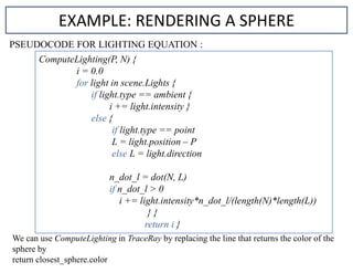
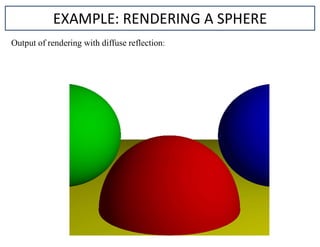
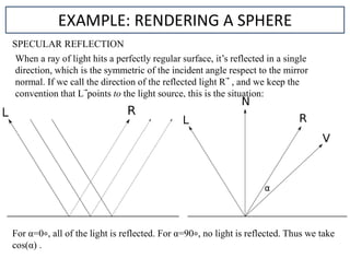
This document provides an overview of ray tracing techniques for computer graphics rendering. It discusses the basic ray tracing algorithm and how it traces the path of light rays in a scene. It covers key concepts like backward ray tracing, shadow rays, reflection rays, refraction, and the basic steps of a ray tracing program. It also provides an example of how to render a sphere using ray tracing by tracing rays from the camera through the image plane and calculating intersections with objects to determine colors.


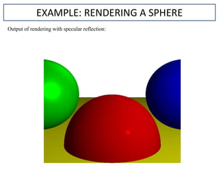
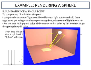
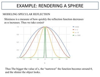
![EXAMPLE: RENDERING A SPHERE
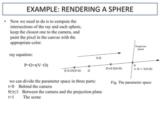
O = <0, 0, 0>
for x in [-Cw/2, Cw/2] {
for y in [-Ch/2, Ch/2] {
D = CanvasToViewport(x, y)
color = TraceRay(O, D, 1, inf)
canvas.PutPixel(x, y, color) } }
CanvasToViewport(x, y) {
return (x*Vw/Cw, y*Vh/Ch, d) }
PSEUDOCODE:
The main method now looks like this:
The CanvasToViewport function is :](https://image.slidesharecdn.com/raytracing-230515104853-7d865636/85/Ray-Tracing-pdf-15-320.jpg)
![EXAMPLE: RENDERING A SPHERE
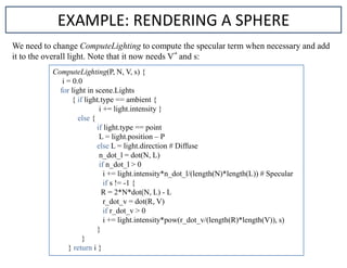
The TraceRay method computes the intersection of the ray with every
sphere, and returns the color of the sphere at the nearest intersection
which is inside the requested range of t:
TraceRay(O, D, t_min, t_max) {
closest_t = inf
closest_sphere = NULL
for sphere in scene.Spheres {
t1, t2 = IntersectRaySphere(O, D, sphere)
if t1 in [t_min, t_max] and t1 < closest_t
closest_t = t1
closest_sphere = sphere
if t2 in [t_min, t_max] and t2 < closest_t
closest_t = t2 closest_sphere = sphere }
if closest_sphere == NULL
return BACKGROUND_COLOR
return closest_sphere.color }
finally, IntersectRaySphere just solves the quadratic equation:](https://image.slidesharecdn.com/raytracing-230515104853-7d865636/85/Ray-Tracing-pdf-16-320.jpg)

![TRACERAY WITH SPECULAR REFLECTION:
TraceRay(O, D, t_min, t_max) {
closest_t = inf
closest_sphere = NULL
for sphere in scene.Spheres {
t1, t2 = IntersectRaySphere(O, D, sphere)
if t1 in [t_min, t_max] and t1 < closest_t
closest_t = t1
closest_sphere = sphere
if t2 in [t_min, t_max] and t2 < closest_t
closest_t = t2
closest_sphere = sphere }
if closest_sphere == NULL
return BACKGROUND_COLOR
P = O + closest_t*D # Compute intersection
N = P - closest_sphere.center # Compute sphere normal at intersection
N = N / length(N)
return closest_sphere.color*ComputeLighting(P, N, -D, sphere.specular)
}
EXAMPLE: RENDERING A SPHERE](https://image.slidesharecdn.com/raytracing-230515104853-7d865636/85/Ray-Tracing-pdf-32-320.jpg)