This document provides an overview of linear algebra, ordinary differential equations, and integral transforms taught in a course at National University of Sciences & Technology. It introduces the Laplace transform, a method for solving initial value problems by transforming differential equations into algebraic equations. Examples show how to take the Laplace transform of basic functions and use properties like shifting to solve problems. The document also discusses the inverse Laplace transform and applications of the method.

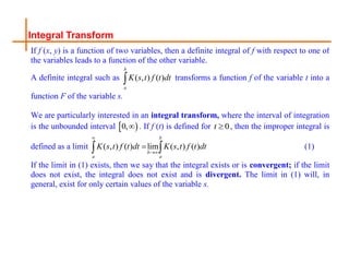
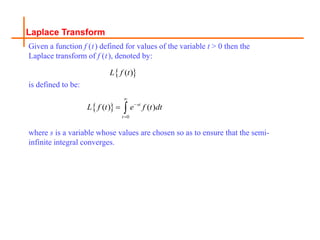
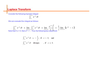
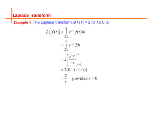
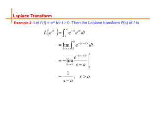
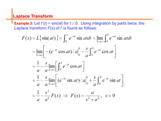
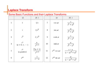
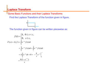
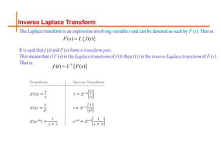
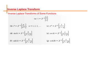
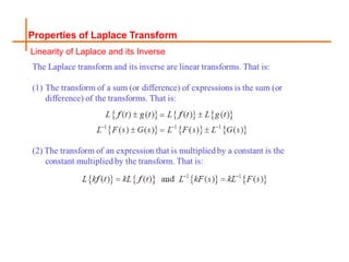
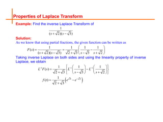
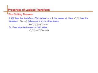
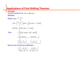
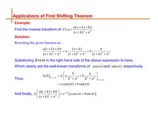
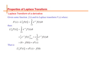
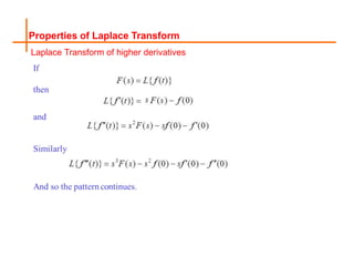
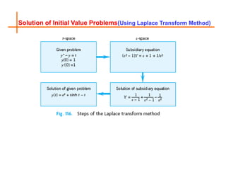
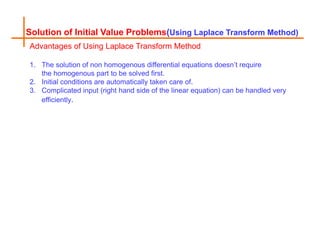
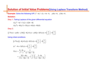
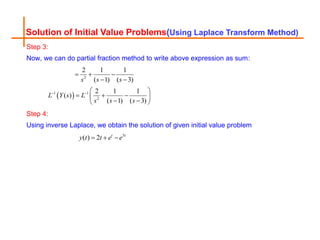
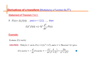
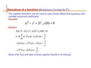
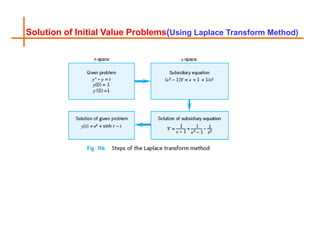
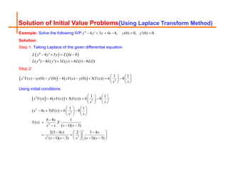
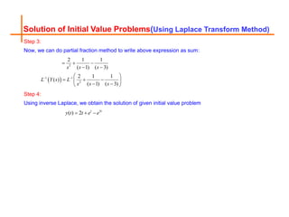
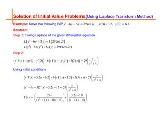
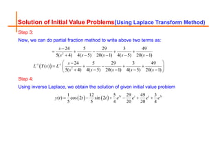
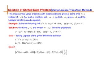
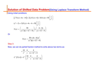
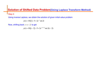
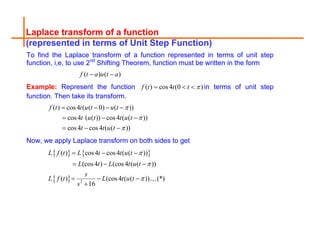
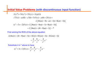
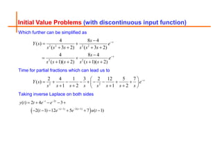
1. 1
1
Linear Algebra & Ordinary Differential Equations
MATH-121
National University of Sciences & Technology (NUST)
School of Electrical Engineering and Computer Science (SEECS)
Department of Basic Sciences
Course Instructor: Dr Saira Zainab
Ph. # 03325193283
Email: saira.zainab@seecs.edu.pk
Office # 207, IAEC
Lecture # 37

2. Integral Transform
If f (x, y) is a function of two variables, then a definite integral of f with respect to one of
the variables leads to a function of the other variable.
A definite integral such as ( , ) ( )
b
a
K s t f t dt
 transforms a function f of the variable t into a
function F of the variable s.
We are particularly interested in an integral transform, where the interval of integration
is the unbounded interval  
0, . If f (t) is defined for 0
t  , then the improper integral is
defined as a limit ( , ) ( ) lim ( , ) ( )
b
b
a a
K s t f t dt K s t f t dt



  (1)
If the limit in (1) exists, then we say that the integral exists or is convergent; if the limit
does not exist, the integral does not exist and is divergent. The limit in (1) will, in
general, exist for only certain values of the variable s.

3. Laplace Transform
Given a function f (t) defined for values of the variable t > 0 then the
Laplace transform of f (t), denoted by:
is defined to be:
where s is a variable whose values are chosen so as to ensure that the semi-
infinite integral converges.
 
( )
L f t
 
0
( ) ( )
st
t
L f t e f t dt



 

4. Laplace Transform

5. Example 1: The Laplace transform of f (t) = 2 for t ≥ 0 is:
Laplace Transform

6. Example 2: Let f (t) = eat for t  0. Then the Laplace transform F(s) of f is
Laplace Transform

7. Example 3: Let f (t) = sin(at) for t  0. Using integration by parts twice, the
Laplace transform F(s) of f is found as follows:
Laplace Transform

8. Laplace Transform
Some Basic Functions and their Laplace Transforms

9. Laplace Transform
Some Basic Functions and their Laplace Transforms
Find the Laplace Transform of the function given in figure.
, 0 ,
( )
0, ,
k x c
f t
x c
 

 


The function given in figure can be written piecewise as:
0
0
0
0
( ) ( ) ( )
( ) ( )
0
(1 )
st
c
st st
c
c
c
st st
sc
F s L f e f t dt
e f t dt e f t dt
k
k e dt e
s
k e
s



 
 

 
 
   



 


10. Inverse Laplace Transform
 
( ) ( )
F s L f t

 
1
( ) ( )
f t L F s



11. Inverse Laplace Transform
Inverse Laplace Transforms of Some Functions

12. Properties of Laplace Transform
Linearity of Laplace and its Inverse

13. Properties of Laplace Transform
Example: Find the inverse Laplace Transform of
1
( 2)( 3)
s s
 
Solution:
As we know that using partial fractions, the given function can be written as
1 1 1 1
( )
( 2)( 3) 2 3 3 2
F s
s s s s
 
  
 
    
 
Taking inverse Laplace on both sides and using the linearity property of inverse
Laplace, we obtain
 
1 1 1
3 2
1 1 1
( )
2 3 3 2
1
( )
2 3
t t
L F s L L
s s
f t e e
  

 
   
 
 
   
  
 
 
 
 


14. Properties of Laplace Transform
First Shifting Theorem
If f(t) has the transform F(s) (where s > k for some k), then ( )
at
e f t has the
transform ( )
F s a
 (where s-a > k ). In other words,
( ( )) ( )
at
L e f t F s a
 
Or, if we take the inverse on both sides,
1
( ) ( ( ))
at
e f t L F s a

 

15. Applications of First Shifting Theorem
Example:
Find the transform of ( ) sinh cos
f t t t

Solution:
Recall sinh
2
t t
e e
t



Then
 
 
   
 
   
 
1 1
2 2 2 2
1 1
1
( ) cos cos cos
2 2
1
( ( )) cos cos
2
1
cos cos
2
1
cos cos
2
1
2 1 1
t t
t t
t t
t t
s s s s
s s s s
e e
f t t e t e t
L f t L e t e t
L e t L e t
L t L t
s s
s s




   
   
 

  
 
 
 
 
 
 
   
 
 
   
 
   
 
Now we can do the due substitution.
   
2 2
2 2
1 ( 1) ( 1)
2 1 1 1 1
s s
s s
 
 
 
 
 
   
 
 

16. Applications of First Shifting Theorem
Example:
Find the inverse transform of 2 2
( )
( )
( )
a s k b
F s
s k


 

 
.
Solution:
Rewriting the given function as
2 2 2 2 2 2
( ) ( )
( ) ( ) ( )
a s k b s k
a b
s k s k s k
 
  
  
 
     
Substituting S=s+k in the right hand side of the above expression to have,
Which clearly are the well-known transforms of cos( )
t
 and sin( )
t
 respectively.
Thus, 2 2 2 2
( )
cos( ) sin( )
S s k
S s k
S
L S L a b
S S
a t b t

 
 
 
 
 
 
 
 
 
 
And finally,  
2 2
( )
cos sin
( )
kt
a s k b
L e a t b t
s k

 


 
 
 
 
 
 

17. Properties of Laplace Transform
Laplace Transform of a derivative

18. Properties of Laplace Transform
Laplace Transform of higher derivatives

19. Solution of Initial Value Problems(Using Laplace Transform Method)

20. Solution of Initial Value Problems(Using Laplace Transform Method)
Advantages of Using Laplace Transform Method
1. The solution of non homogenous differential equations doesn’t require
the homogenous part to be solved first.
2. Initial conditions are automatically taken care of.
3. Complicated input (right hand side of the linear equation) can be handled very
efficiently.

21. Solution of Initial Value Problems(Using Laplace Transform Method)
Example: Solve the following IVP 4 3 6 8, (0) 0, (0) 0
y y y t y y
  
      .
Solution:
Step 1: Taking Laplace of the given differential equation
   
4 3 6 8
( ) 4 ( ) 3 ( ) 6 ( ) 8 (1)
L y y y L t
L y L y L y L t L
 
   
 
   
Step 2:
   
2
2
1 1
( ) (0) (0) 4 ( ) (0) 3( ( )) 6 8
s Y s sy y sY s y Y s
s s
   

      
   
   
Using initial conditions
   
2
2
2
2
2
2 2
1 1
( ) 4 ( ) 3( ( )) 6 8
1 1
( 4 3) ( ) 6 8
6 8 1
( )
( 1)( 3)
2(3 4 ) 2 3 4
( 1)( 3) ( 1)( 3)
s Y s sY s Y s
s s
s s Y s
s s
s
Y s X
s s s s
s s
s s s s s s
   
   
   
   
   
   
   
   


  
 
 
 
   
 
   
  

22. Solution of Initial Value Problems(Using Laplace Transform Method)
Step 3:
Now, we can do partial fraction method to write above expression as sum:
 
2
1 1
2
2 1 1
( 1) ( 3)
2 1 1
( )
( 1) ( 3)
s s s
L Y s L
s s s
 
  
 
 
  
 
 
 
Step 4:
Using inverse Laplace, we obtain the solution of given initial value problem
3
( ) 2 t t
y t t e e
  

23. Derivatives of a transform (Multiplying a Function By tn )
Statement of Theorem 7.4.1:
If , and n = 1,2,3, …, then
Example:
( ) ( ( ))
F s L f t

{ ( )} ( 1) ( )
n
n n
n
d
L t f t F s
ds
 

24. Derivatives of a transform (Multiplying a Function By tn )
The Laplace transform can be used to solve linear differential equations with
variable monomial coefficients
Example:
Solution:
Solve it for Y(s) and take inverse Laplace transform to find y(t).
2
2 , (0) 0
ty y t y
 
  
2
2
3
2
3
2
3
( ) ( ) (2 ), (0) 0
2
( 1) ( ( )) ( ( ))
2
2 ( ) ( ) ( )
2
( ) 3 ( )
L ty L y L t y
d
s Y s sY s
ds s
sY s s Y s sY s
s
s Y s sY s
s
 
  
  

   

  

25. Solution of Initial Value Problems(Using Laplace Transform Method)

26. Solution of Initial Value Problems(Using Laplace Transform Method)
Advantages of Using Laplace Transform Method
1. The solution of non homogenous differential equations doesn’t require
the homogenous part to be solved first.
2. Initial conditions are automatically taken care of.
3. Complicated input (right hand side of the linear equation) can be handled very
efficiently.

27. Solution of Initial Value Problems(Using Laplace Transform Method)
Example: Solve the following IVP 4 3 6 8, (0) 0, (0) 0
y y y t y y
  
      .
Solution:
Step 1: Taking Laplace of the given differential equation
   
4 3 6 8
( ) 4 ( ) 3 ( ) 6 ( ) 8 (1)
L y y y L t
L y L y L y L t L
 
   
 
   
Step 2:
   
2
2
1 1
( ) (0) (0) 4 ( ) (0) 3( ( )) 6 8
s Y s sy y sY s y Y s
s s
   

      
   
   
Using initial conditions
   
2
2
2
2
2
2 2
1 1
( ) 4 ( ) 3( ( )) 6 8
1 1
( 4 3) ( ) 6 8
6 8 1
( )
( 1)( 3)
2(3 4 ) 2 3 4
( 1)( 3) ( 1)( 3)
s Y s sY s Y s
s s
s s Y s
s s
s
Y s X
s s s s
s s
s s s s s s
   
   
   
   
   
   
   
   


  
 
 
 
   
 
   
  

28. Solution of Initial Value Problems(Using Laplace Transform Method)
Step 3:
Now, we can do partial fraction method to write above expression as sum:
 
2
1 1
2
2 1 1
( 1) ( 3)
2 1 1
( )
( 1) ( 3)
s s s
L Y s L
s s s
 
  
 
 
  
 
 
 
Step 4:
Using inverse Laplace, we obtain the solution of given initial value problem
3
( ) 2 t t
y t t e e
  

29. Solution of Initial Value Problems(Using Laplace Transform Method)
Example: Solve the following IVP 6 5 29cos2 , (0) 3.2, (0) 6.2
y y y t y y
  
     .
Solution:
Step 1: Taking Laplace of the given differential equation
   
6 5 29cos2
( ) 6 ( ) 5 ( ) 29 (cos2 )
L y y y L t
L y L y L y L t
 
  
 
  
Step 2:
   
2
2
( ) (0) (0) 6 ( ) (0) 5( ( )) 29
4
s
s Y s sy y sY s y Y s
s
 

       

 
Using initial conditions
   
2
2
2
2
2
( ) 3.2 6.2 6 ( ) 3.2 5( ( )) 29
4
( 6 5) ( ) 3.2 13 29
4
29 3.2 13
( )
( 4)( 1)( 5) ( 1)( 5)
s
s Y s s sY s Y s
s
s
s s Y s s
s
s s
Y s
s s s s s
 
       

 
 
      

 
   

 
   
    
   

30. Solution of Initial Value Problems(Using Laplace Transform Method)
Step 3:
Now, we can do partial fraction method to write above two terms as:
 
2
1 1
2
24 5 29 3 49
5( 4) 4( 5) 20( 1) 4( 5) 20( 1)
24 5 29 3 49
( )
5( 4) 4( 5) 20( 1) 4( 5) 20( 1)
s
s s s s s
s
L Y s L
s s s s s
 

    
    
 

    
 
    
 
Step 4:
Using inverse Laplace, we obtain the solution of given initial value problem
    5 5
1 12 5 29 49 3
( ) cos 2 sin 2
5 5 4 20 20 4
t t t t
y t t t e e e e
     

31. Solution of Shifted Data Problem(Using Laplace Transform Method)
This means initial value problems with initial conditions given at some time 0
t t

instead of 0
t  . For such a problem, set 0
t t t
  so that 0
t t
 gives 0
t  and the
Laplace transform can be applied.
Example: Solve the following IVP 2 5 50 100, (2) 4, (2) 14
y y y t y y
  
       .
Solution: We have 0 2
t  and we set 2
t t
  . Then the problem is
2 5 50( 2) 100, (0) 4, (0) 14
y y y t y y
  
       
Step 1: Taking Laplace of the given differential equation
   
2 5 50
( ) 2 ( ) 5 ( ) 50 ( )
L y y y L t
L y L y L y L t
 
  
 
  
Step 2:
   
2
2
1
( ) (0) (0) 2 ( ) (0) 5( ( )) 50
s Y s sy y sY s y Y s
s
 

       
 

32. Solution of Shifted Data Problem(Using Laplace Transform Method)
Using initial conditions
   
2
2
2
2
2 2 2
1
( ) 4 14 2 ( ) 4 5( ( )) 50
1
( 2 5) ( ) 4 6 50
50 6 4
( )
( )(( 1) 4) ( 1) 4
s Y s s sY s Y s
s
s s Y s s
s
s
Y s
s s s
 
       
 
 
      
 
   

 
   
   
   
Or
2
2 2
50 (6 4 )
( )
( )(( 1) 4)
s s
Y s
s s
 

 
Step 3:
Now, we can do partial fraction method to write above two terms as:
 
2 2
1 1
2 2
10 4 4
( 1) 4
10 4 4
( )
( 1) 4
s s s
L Y s L
s s s
 
  
 
 
  
 
 
 

33. Solution of Shifted Data Problem(Using Laplace Transform Method)
Step 4:
Using inverse Laplace, we obtain the solution of given initial value problem
 
( ) 10 5 2 sin2
t
y t t e t

  
Now, shifting back 2
t t
  to get
  ( 2)
( ) 10 2 5 2 sin2( 2)
t
y t t e t
 
    

34. Unit Step Function (Heaviside Function)
Definition: The unit step function or Heaviside function ( )
u t a
 has a jump of
size 1 at t a
 and is defined as
0,
( )
1,
if t a
u t a
if t a


  


The Laplace transform of ( )
u t a
 follows from the definition as an integral
0 0
( ( )) ( ) .1
st sa
st st
a
e e
L u t a e u t a dt e dt
s s

   
 
     
 
Second Shifting Theorem:
If ( )
f t has the transform ( )
F s then the shifted function
0,
( ) ( ) ( )
( ),
if t a
f f t a u t a
f t a if t a



    
 

has the transform ( )
as
e F s

. That is, if  
( ) ( )
L f t F s
 , then
 
( ) ( ) ( )
as
L f t a u t a e F s

  
If we take the inverse on both sides, we can write
 
1
( ) ( ) ( )
as
f t a u t a L e F s
 
  

35. Representation of a function in terms of Unit Step Function
One of the major applications of Unit step function is to write a piecewise
discontinuous function in terms of unit step.
But before going to this representation, we need to understand what we mean by
the difference of two unit step functions.
Example: Given two unit step functions
0, 1 0, 3
( 1) ( 3)
1, 1 1, 3
if t if t
u t and u t
if t if t
 
 
   
 
 
 
The difference function ( 1) ( 3)
u t u t
   is given as
0, 1
( 1) ( 3) 1, 1 3
0, 3
if t
u t u t if t
if t



     

 

.
More generally, if 0 a b
 
0,
( ) ( ) 1,
0,
if t a
u t a u t b if a t b
if t b



     

 


36. Representation of a function in terms of Unit Step Function
i.e. if ( )
g t is any function to be represented in terms of unit step function, then
 
0,
( ) ( ) ( ) ( ),
0,
if t a
g t u t a u t b g t if a t b
if t b



     

 

Example: Write the function defined as
2 , 0 1
4 2 , 1 2
( )
0, 2 3
1, 3.
t if t
t if t
f t
if t
if t
 

   

 
 

 

using unit step function.
Solution: It will be written as
    
   
( ) 2 ( 0) ( 1) 4 2 ( 1) ( 2)
0 ( 2) ( 3) 1 ( 3)
f t t u t u t t u t u t
u t u t u t
        
     

37. Laplace transform of a function
(represented in terms of Unit Step Function)
To find the Laplace transform of a function represented in terms of unit step
function, i,e, to use 2nd
Shifting Theorem, function must be written in the form
( ) ( )
f t a u t a
 
Example: Represent the function ( ) cos4 (0 )
f t t t 
   in terms of unit step
function. Then take its transform.
( ) cos4 ( ( 0) ( ))
cos4 ( ( )) cos4 ( ( ))
cos4 cos4 ( ( ))
f t t u t u t
t u t t u t
t t u t



   
  
  
Now, we apply Laplace transform on both sides to get
   
  2
( ) cos4 cos4 ( ( ))
(cos4 ) (cos4 ( ( ))
( ) (cos4 ( ( )) (*)
16
L f t L t t u t
L t L t u t
s
L f t L t u t
s



  
  
  


38. Laplace transform of a function
(represented in terms of Unit Step Function)
Now, we have to apply second shifting theorem on 2nd
part of (*). For that, we
must write it as
(cos4 ( ( )) ( ) ( )
t u t f t u t
  
   
On comparison, cos4 ( )
t f t 
  . So, substitute
t
t
 
 
 
 
.
Thus
2
cos 4( ) ( )
( ( )) (cos 4( )) (cos 4 )
( )
16
f
L f L L
s
F s
s
  
   
 
  
 

So finally, 2
(cos4 ( ( ))
16
s s
L t u t e
s

 
 

.
Put it in (*) to get
  2 2
2
( )
16 16
(1 )
16
s
s
s se
L f t
s s
s
e
s




 
 
 


39. Laplace transform of a function
(represented in terms of Unit Step Function)
Example: Represent the function 2
( ) (1 2)
f t t t
   in terms of unit step function.
Then take its transform.
2
2 2
( ) ( ( 1) ( 2))
( 1) ( 2)
f t t u t u t
t u t t u t
   
   
Now, we apply Laplace transform on both sides to get
   
2 2
2 2
( ) ( 1) ( 2)
( ( 1)) ( ( 2)) (*)
L f t L t u t t u t
L t u t L t u t
   
   
Now, we have to apply second shifting theorem on both the terms of (*). For that, we
must write them as
2 2
( ( 1)) ( 1) ( 1) ( ( 2)) ( 2) ( 2)
t u t f t u t and t u t f t u t
       
On comparison, 2 2
( 1) ( 2)
t f t and t f t
   
So, substitute
1
1
t
t


 
 
and
2
2
t
t


 
 

40. Laplace transform of a function
(represented in terms of Unit Step Function)
Thus 2 2
( 1) ( ) ( 2) ( )
f and f
   
   
So finally,
 
2
2
3 2
( ( )) ( 1)
( 2 1)
2 2 1
( )
L f L
L
F s
s s s
 
 
 
  
   
and
 
2
2
3 2
( ( )) ( 2)
( 4 4)
2 4 4
( )
L f L
L
F s
s s s
 
 
 
  
   
Put it in (*) to get
  2
3 2 3 2
2 2 1 2 4 4
( ) s s
L f t e e
s s s s s s
 
   
     
   
   

41. Inverse Laplace transform of a function
(Using 2nd Shifting Theorem)
Recall that if  
( ) ( )
L f t F s
 , then
 
( ) ( ) ( )
as
L f t a u t a e F s

  
If we take the inverse on both sides, we can write
 
1
( ) ( ) ( )
as
f t a u t a L e F s
 
  
Example: Find ( )
f t , if  
L f equals
(a).
3
2
2( )
4
s s
e e
s
 


(b).
 
2 ( 1)
2
(1 )( 1)
( 1) 1
s
e s
s

 
 
 

42. Inverse Laplace transform of a function
(Using 2nd Shifting Theorem)
(a). Using 2nd
Shifting theorem and inverse Laplace of sinh, we obtain
3
2
3
1 1
2 2
1 1 3
2 2
2( )
( )
4
2 2
4 4
2 2
4 4
sinh(2( 1))( ( 1)) sinh(2( 3))( ( 3))
s s
s s
s s
e e
L f
s
e e
f L L
s s
L e L e
s s
t u t t u t
 
 
 
   



   
 
   
 
   
   
 
   
 
   
     

43. Inverse Laplace transform of a function
(Using 2nd Shifting Theorem)
(b). Rewrite the given function as
2
2 2
( ) ,
1 1
S
S Se
G S
S S


 
 
where ( ) ( 1)
G S F s
 
Then using the inverse Laplace and 2nd
shifting theorem, we have
( ) cos( ) ( ) cos( 2 ) ( 2 )
cos( ) ( ) cos( ) ( 2 )
cos( )( ( ) ( 2 ))
g t t u t t u t
t u t t u t
t u t u t
 


   
  
  
Thus ( ) cos ( ( ) ( 2 ))
t
f t e t u t u t 

   .

44. Initial Value Problems (with discontinuous input function)
Example: Solve the given initial value problem
3 2 4 0 1 8 1
(0) 0, (0) 0
y y y t if t and if t
y y
 
     

 
Solution: Given differential equation can be re written as
3 2 ( )
( ) 4 0 1
8 1
y y y g t
where g t t if t
if t
 
  
  
 
Using Laplace to solve this problem, we apply it on both sides.
 
3 2 ( ( ))
L y y y L g t
 
  
We will use linearity of Laplace transform, transforms of derivative terms, initial
conditions on the LHS of the above equation and unit step function on the RHS
of the equation.

45. Initial Value Problems (with discontinuous input function)
 
 
 
2
2
( ) 3 ( ) 2 ( ) ( ( ))
( ) (0) (0) 3 ( ) (0) 2 ( )
4 ( ( 0) ( 1)) 8( ( 1))
( 3 2) ( ) 4 ( ) 4 ( 1) 8( ( 1))
4 ( ) (4 8) ( 1) *
L y L y L y L g t
s Y s sy y sY s y Y s
L t u t u t u t
s s Y s L tu t tu t u t
L tu t t u t
 
  

     
    
      
   
First solving the RHS of the above equation
2 2
(4 ( ) (4 8) ( 1)) 4 ( ) 8 ( ( 1)) 4 ( ( 1))
4 8 4
s s
L tu t t u t L t L u t L tu t
e e
s s s
 
       
  
Substitute it in * above to have
2
2 2
4 8 4
( 3 2) ( ) s s
s s Y s e e
s s s
 
    

46. Initial Value Problems (with discontinuous input function)
Which further can be simplified as
2 2 2 2
2 2
4 8 4
( )
( 3 2) ( 3 2)
4 8 4
( 1)( 2) ( 1)( 2)
s
s
s
Y s e
s s s s s s
s
e
s s s s s s



 
   

 
   
Time for partial fractions which can lead us to
2 2
2 4 1 3 2 12 5 7
( )
1 2 1 2
s
Y s e
s s s s s s s s

 
        
 
   
 
Taking inverse Laplace on both sides
 
2
( 1) 2( 1)
( ) 2 4 3
2( 1) 12 5 7 ( 1)
t t
t t
y t t e e
t e e u t
 
   
    
     