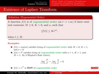
This document provides an introduction and overview of Laplace transforms. It begins with background on integral transforms and discusses how the Laplace transform specifically is used to transform differential equations from the time domain to the complex frequency domain for algebraic manipulation. The document then covers properties of the Laplace transform like linearity and examples of calculating Laplace transforms. It also discusses prerequisites like existence conditions and concludes with a short table of common Laplace transform pairs.

![Introduction
Laplace Transforms
Short Table of Laplace Transforms
Properties of Laplace Transform
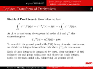
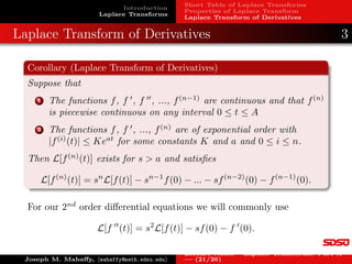
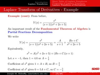
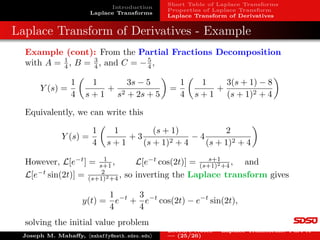
Laplace Transform of Derivatives
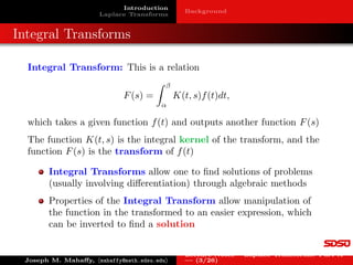
Laplace Transform
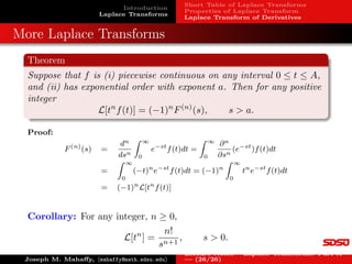
Definition (Laplace Transform)
Let f be a function on [0, ∞). The Laplace transform of f is the
function F defined by the integral,
F(s) =
Z ∞
0
e−st
f(t)dt.
The domain of F(s) is the set of all values of s for which this integral
converges. The Laplace transform of f is denoted by both F and
L.
Convention uses s as the independent variable and capital letters for
the transformed functions:
L[f] = F L[y] = Y L[x] = X
L[f](s) = F(s) L[y](s) = Y (s) L[x](s) = X(s)
Joseph M. Mahaffy, hmahaffy@math.sdsu.edui
Lecture Notes – Laplace Transforms: Part A
— (7/26)](https://image.slidesharecdn.com/laplaceappt-220811190011-d2c66460/85/LaplaceA-ppt-pdf-11-320.jpg)
![Introduction
Laplace Transforms
Short Table of Laplace Transforms
Properties of Laplace Transform
Laplace Transform of Derivatives
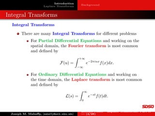
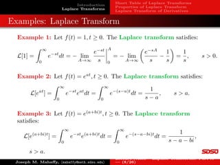
Examples: Laplace Transform
Example 1: Let f(t) = 1, t ≥ 0. The Laplace transform satisfies:
L[1] =
Z ∞
0
e−st
dt = − lim
A→∞
e−st
s](https://image.slidesharecdn.com/laplaceappt-220811190011-d2c66460/85/LaplaceA-ppt-pdf-12-320.jpg)
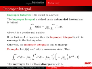
![A
0
= − lim
A→∞
e−sA
s
−
1
s
=
1
s
, s 0.
Example 2: Let f(t) = eat
, t ≥ 0. The Laplace transform satisfies:
L[eat
] =
Z ∞
0
e−st
eat
dt =
Z ∞
0
e−(s−a)t
dt =
1
s − a
, s a.
Example 3: Let f(t) = e(a+bi)t
, t ≥ 0. The Laplace transform
satisfies:
L[e(a+bi)t
] =
Z ∞
0
e−st
e(a+bi)t
dt =
Z ∞
0
e−(s−a−bi)t
dt =
1
s − a − bi
,
s a.
Joseph M. Mahaffy, hmahaffy@math.sdsu.edui
Lecture Notes – Laplace Transforms: Part A
— (8/26)](https://image.slidesharecdn.com/laplaceappt-220811190011-d2c66460/85/LaplaceA-ppt-pdf-16-320.jpg)
![Introduction
Laplace Transforms
Short Table of Laplace Transforms
Properties of Laplace Transform
Laplace Transform of Derivatives
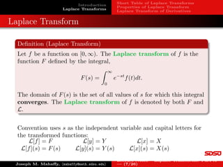
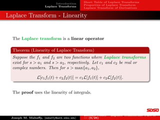
Laplace Transform - Linearity
The Laplace transform is a linear operator
Theorem (Linearity of Laplace Transform)
Suppose the f1 and f2 are two functions where Laplace transforms
exist for s a1 and s a2, respectively. Let c1 and c2 be real or
complex numbers. Then for s max{a1, a2},
L[c1f1(t) + c2f2(t)] = c1L[f1(t)] + c2L[f2(t)].
The proof uses the linearity of integrals.
Joseph M. Mahaffy, hmahaffy@math.sdsu.edui
Lecture Notes – Laplace Transforms: Part A
— (9/26)](https://image.slidesharecdn.com/laplaceappt-220811190011-d2c66460/85/LaplaceA-ppt-pdf-17-320.jpg)
![Introduction
Laplace Transforms
Short Table of Laplace Transforms
Properties of Laplace Transform
Laplace Transform of Derivatives
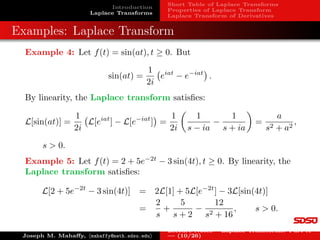
Examples: Laplace Transform
Example 4: Let f(t) = sin(at), t ≥ 0. But
sin(at) =
1
2i
eiat
− e−iat
.
By linearity, the Laplace transform satisfies:
L[sin(at)] =
1
2i
L[eiat
] − L[e−iat
]
=
1
2i
1
s − ia
−
1
s + ia
=
a
s2 + a2
,
s 0.
Example 5: Let f(t) = 2 + 5e−2t
− 3 sin(4t), t ≥ 0. By linearity, the
Laplace transform satisfies:
L[2 + 5e−2t
− 3 sin(4t)] = 2L[1] + 5L[e−2t
] − 3L[sin(4t)]
=
2
s
+
5
s + 2
−
12
s2 + 16
, s 0.
Joseph M. Mahaffy, hmahaffy@math.sdsu.edui
Lecture Notes – Laplace Transforms: Part A
— (10/26)](https://image.slidesharecdn.com/laplaceappt-220811190011-d2c66460/85/LaplaceA-ppt-pdf-18-320.jpg)
![Introduction
Laplace Transforms
Short Table of Laplace Transforms
Properties of Laplace Transform
Laplace Transform of Derivatives
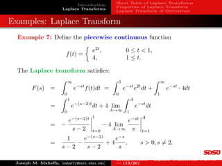
Examples: Laplace Transform
Example 6: Let f(t) = t cos(at), t ≥ 0. The Laplace transform
satisfies:
L[t cos(at)] =
Z ∞
0
e−st
t cos(at)dt =
1
2
Z ∞
0
te−(s−ia)t
+ te−(s+ia)t
dt.
Integration by parts gives
Z ∞
0
te−(s−ia)t
dt =
te−(s−ia)t
s − ia
+
e−(s−ia)t
(s − ia)2
∞
0
=
1
(s − ia)2
, s 0.
Similarly, Z ∞
0
te−(s+ia)t
dt =
1
(s + ia)2
, s 0.
Thus,
L[t cos(at)] =
1
2
1
(s − ia)2
+
1
(s + ia)2
=
s2
− a2
(s2 + a2)2
, s 0.
Joseph M. Mahaffy, hmahaffy@math.sdsu.edui
Lecture Notes – Laplace Transforms: Part A
— (11/26)](https://image.slidesharecdn.com/laplaceappt-220811190011-d2c66460/85/LaplaceA-ppt-pdf-19-320.jpg)