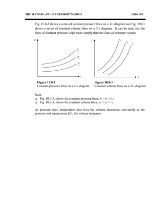
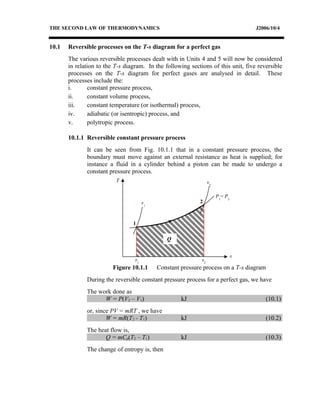
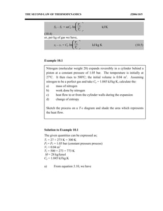
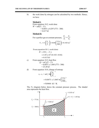
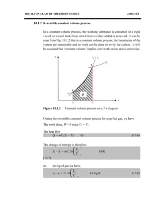
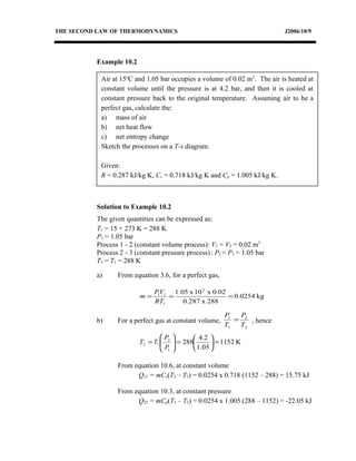
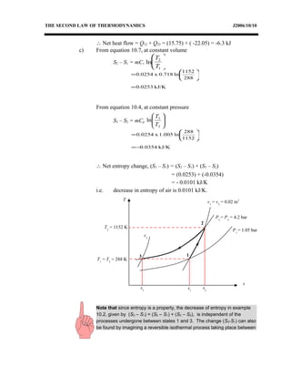
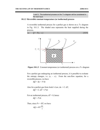
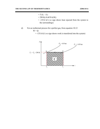
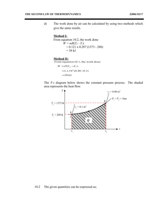
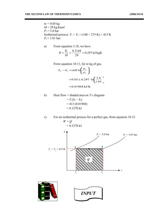
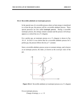
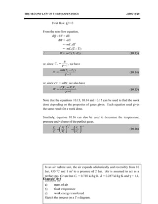
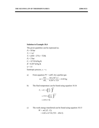
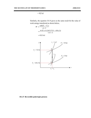
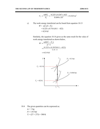
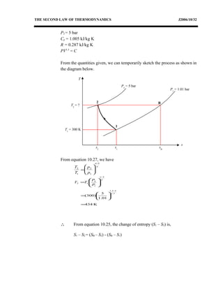
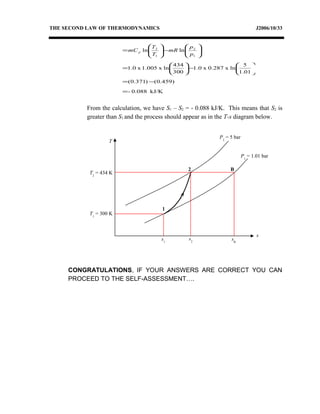
SlideShare a Scribd company logo
THE SECOND LAW OF THERMODYNAMICS J2006/10/1
THE SECOND LAW OF THERMODYNAMICS
OBJECTIVES
General Objective : To define and explain the Second Law of Thermodynamics and
perform calculations involving the expansion and compression of
perfect gases.
Specific Objectives : At the end of the unit you will be able to:
 sketch the processes on a temperature-entropy diagram
 calculate the change of entropy, work and heat transfer of
perfect gases in reversible processes at:
i. constant pressure process
ii. constant volume process
iii. constant temperature (or isothermal) process
iv. adiabatic (or isentropic) process
v. polytropic process
UNIT 10
THE SECOND LAW OF THERMODYNAMICS J2006/10/2
10.0 The P-V and T-s diagram for a perfect gas
Property diagrams serve as great visual aids in the thermodynamic analysis of
processes. We have used P-V and T-s diagrams extensively in the previous unit
showing steam as a working fluid. In the second law analysis, it is very helpful to
plot the processes on diagrams which coordinate the entropy. The two diagrams
commonly used in the second law analysis are the pressure-volume and
temperature-entropy.
Fig. 10.0-1 shows a series of constant temperature lines on a P-V diagram. The
constant temperature lines, T3 > T2 > T1 are shown.
Figure 10.0-1 The constant temperature lines on a P-V diagram for a perfect gas
Since entropy is a property of a system, it may be used as a coordinate, with
temperature as the other ordinate, in order to represent various cycles graphically. It
is useful to plot lines of constant pressure and constant volume on a T-s diagram for
a perfect gas. Since changes of entropy are of more direct application than the
absolute value, the zero of entropy can be chosen at any arbitrary reference
temperature and pressure.
INPUTINPUT
T3 > T2 > T1
P
V
T1
T2
T3
Constant temperature lines
THE SECOND LAW OF THERMODYNAMICS J2006/10/3
Fig. 10.0-2 shows a series of constant pressure lines on a T-s diagram and Fig.10.0-3
shows a series of constant volume lines on a T-s diagram. It can be seen that the
lines of constant pressure slope more steeply than the lines of constant volume.
Note:
 Fig. 10.0-2, shows the constant pressure lines, P3 > P2 > P1;
 Fig. 10.0-3, shows the constant volume lines, v1 > v2 > v3.
As pressure rises, temperature also rises but volume decreases; conversely as the
pressure and temperature fall, the volume increases.
T
s
P1
P2
P3
Figure 10.0-2
Constant pressure lines on a T-s diagram
T
s
v2
v1
v3
Figure 10.0-3
Constant volume lines on a T-s diagram
THE SECOND LAW OF THERMODYNAMICS J2006/10/4
10.1 Reversible processes on the T-s diagram for a perfect gas
The various reversible processes dealt with in Units 4 and 5 will now be considered
in relation to the T-s diagram. In the following sections of this unit, five reversible
processes on the T-s diagram for perfect gases are analysed in detail. These
processes include the:
i. constant pressure process,
ii. constant volume process,
iii. constant temperature (or isothermal) process,
iv. adiabatic (or isentropic) process, and
v. polytropic process.
10.1.1 Reversible constant pressure process
It can be seen from Fig. 10.1.1 that in a constant pressure process, the
boundary must move against an external resistance as heat is supplied; for
instance a fluid in a cylinder behind a piston can be made to undergo a
constant pressure process.
During the reversible constant pressure process for a perfect gas, we have
The work done as
W = P(V2 – V1) kJ (10.1)
or, since PV = mRT , we have
W = mR(T2 - T1) kJ (10.2)
The heat flow is,
Q = mCp(T2 – T1) kJ (10.3)
The change of entropy is, then
T
s
P1
= P2
v2
v1
1
2
s1
s2
Q
Figure 10.1.1 Constant pressure process on a T-s diagram
Nitrogen (molecular weight 28) expands reversibly in a cylinder behind a
piston at a constant pressure of 1.05 bar. The temperature is initially at
27o
C. It then rises to 500o
C; the initial volume is 0.04 m3
. Assuming
nitrogen to be a perfect gas and take Cp = 1.045 kJ/kg K, calculate the:
a) mass of nitrogen
b) work done by nitrogen
c) heat flow to or from the cylinder walls during the expansion
d) change of entropy
Sketch the process on a T-s diagram and shade the area which represents
the heat flow.
THE SECOND LAW OF THERMODYNAMICS J2006/10/5
S2 – S1 = mCp ln
T
T
2
1





 kJ/K
(10.4)
or, per kg of gas we have,
s2 – s1 = Cp ln
T
T
2
1





 kJ/kg K (10.5)
Example 10.1
Solution to Example 10.1
The given quantities can be expressed as;
T1 = 27 + 273 K = 300 K
P1 = P2 = 1.05 bar (constant pressure process)
V1 = 0.04 m3
T2 = 500 + 273 = 773 K
M = 28 kg/kmol
Cp = 1.045 kJ/kg.K
a) From equation 3.10, we have
THE SECOND LAW OF THERMODYNAMICS J2006/10/6
kg0.0471
300x0.297
0.04x10x1.05
havewe,=sinceThen
KkJ/kg0.297
28
3144.8
2
1
11
===
===
RT
VP
m
mRTPV
M
R
R o
THE SECOND LAW OF THERMODYNAMICS J2006/10/7
b) the work done by nitrogen can be calculated by two methods. Hence,
we have
Method I:
From equation 10.2, work done
W = mR(T2 - T1)
= 0.0471 x 0.297 (773 - 300)
= 6.617 kJ
Method II:
For a perfect gas at constant pressure,
2
2
1
1
T
V
T
V
=
kJ6.615
0.04)-(0.10310x1.05
)(
donework10.1,equationFrom
m0.103
300
773
0.04
2
12
3
1
2
12
=
=
−=
=





=





=
VVPW
T
T
VV
c) From equation 10.3, heat flow
Q = mCp(T2 - T1)
= 0.0471 x 1.045 (773 - 300)
= 23.28 kJ
d) From equation 10.4, change of entropy
s2 - s1 = mCp ln
T
T
2
1






=






=
0.0471 x 1.045 ln
773
300
kJ / K0 0466.
The T-s diagram below shows the constant pressure process. The shaded
area represents the heat flow.
T
s
P1
= P2
= 1.05 bar
v2
= 0.103 m3
v1
= 0.04 m3
1
2
s1
s2
Q
T1
= 300 K
T2
= 773 K
THE SECOND LAW OF THERMODYNAMICS J2006/10/8
10.1.2 Reversible constant volume process
In a constant volume process, the working substance is contained in a rigid
vessel (or closed tank) from which heat is either added or removed. It can be
seen from Fig. 10.1.2 that in a constant volume process, the boundaries of the
system are immovable and no work can be done on or by the system. It will
be assumed that ‘constant volume’ implies zero work unless stated otherwise.
During the reversible constant volume process for a perfect gas, we have
The work done, W = 0 since V2 = V1.
The heat flow
Q = mCv(T2 – T1) kJ (10.6)
The change of entropy is therefore
S2 – S1 = mCv ln
T
T
2
1





 kJ/K
(10.7)
or, per kg of gas we have,
s2 – s1 = Cv ln
T
T
2
1





 kJ/ kg K (10.8)
T
s
v1
= v2
P1
1
2
s1
s2
Q
P2
Figure 10.1.2 Constant volume process on a T-s diagram
Air at 15o
C and 1.05 bar occupies a volume of 0.02 m3
. The air is heated at
constant volume until the pressure is at 4.2 bar, and then it is cooled at
constant pressure back to the original temperature. Assuming air to be a
perfect gas, calculate the:
a) mass of air
b) net heat flow
c) net entropy change
Sketch the processes on a T-s diagram.
Given:
R = 0.287 kJ/kg K, Cv = 0.718 kJ/kg K and Cp = 1.005 kJ/kg K.
THE SECOND LAW OF THERMODYNAMICS J2006/10/9
Example 10.2
Solution to Example 10.2
The given quantities can be expressed as;
T1 = 15 + 273 K = 288 K
P1 = 1.05 bar
Process 1 - 2 (constant volume process): V1 = V2 = 0.02 m3
Process 2 - 3 (constant pressure process) : P2 = P3 = 1.05 bar
T3 = T1 = 288 K
a) From equation 3.6, for a perfect gas,
kg0.0254
288x0.287
0.02x10x1.05 2
1
11
===
RT
VP
m
b) For a perfect gas at constant volume,
2
2
1
1
T
P
T
P
= , hence
K1152
05.1
2.4
288
1
2
12 =





=





=
P
P
TT
From equation 10.6, at constant volume
Q12 = mCv(T2 – T1) = 0.0254 x 0.718 (1152 – 288) = 15.75 kJ
From equation 10.3, at constant pressure
Q23 = mCp(T3 – T2) = 0.0254 x 1.005 (288 – 1152) = -22.05 kJ
THE SECOND LAW OF THERMODYNAMICS J2006/10/10
∴ Net heat flow = Q12 + Q23 = (15.75) + ( -22.05) = -6.3 kJ
c) From equation 10.7, at constant volume
S2 – S1 = mCv ln
T
T
2
1






From equation 10.4, at constant pressure
S3 – S2 = mCp 





2
3
ln
T
T
∴ Net entropy change, (S3 – S1) = (S2 – S1) + (S3 – S2)
= (0.0253) + (-0.0354)
= - 0.0101 kJ/K
i.e. decrease in entropy of air is 0.0101 kJ/K.
Note that since entropy is a property, the decrease of entropy in example
10.2, given by (S3 – S1) = (S2 – S1) + (S3 – S2), is independent of the
processes undergone between states 1 and 3. The change (S3-S1) can also
be found by imagining a reversible isothermal process taking place between
kJ/K0253.0
288
1152
ln0.718x0.0254
=






=
kJ/K0354.0
1152
288
ln1.005x0.0254
−=






=
T
s
P2
= P3
= 4.2 bar
v1
= v2
= 0.02 m3
v3
3
2
s3
s2
T1
= T3
= 288 K
T2
= 1152 K
1
P1
= 1.05 bar
s1
THE SECOND LAW OF THERMODYNAMICS J2006/10/11
1 and 3. The isothermal process on the T-s diagram will be considered in
the next input.
10.1.3 Reversible constant temperature (or isothermal) process
A reversible isothermal process for a perfect gas is shown on a T-s diagram
in Fig. 10.1.3. The shaded area represents the heat supplied during the
process,
i.e. Q = T(s2 - s1) (10.9)
For a perfect gas undergoing an isothermal process, it is possible to evaluate
the entropy changes, i.e. (s2 – s1). From the non-flow equation, for a
reversible process, we have
dQ = du + P dv
Also for a perfect gas from Joule’s Law, du = Cv dT,
dQ = Cv dT + P dv
For an isothermal process, dT = 0, hence
dQ = P dv
Then, since Pv = RT, we have
v
v
RTQ
d
d =
T
s
P2
v2v1
1 2
s1
s2
Q
Figure 10.1.3 Constant temperature (or isothermal) process on a T-s diagram
P1
T1
= T2
THE SECOND LAW OF THERMODYNAMICS J2006/10/12
Now from equation 9.5
∫∫∫ ===−
2
1
2
1
ddd2
1
12
v
v
v
v v
v
R
Tv
vRT
T
Q
ss
i.e. 





=





=−
2
1
1
2
12 lnln
p
p
R
v
v
Rss kJ/kg K (10.10)
or, for mass, m (kg), of a gas
S2 – S1 = m(s2 – s1)
i.e. 





=





=−
2
1
1
2
12 lnln
p
p
mR
v
v
mRSS kJ/K (10.11)
Therefore, the heat supplied is given by,
( ) 





=





=−=
2
1
1
2
12 lnln
p
p
RT
v
v
RTssTQ
or, for mass, m (kg), of a gas
( ) 





=





=−=
2
1
1
2
12 lnln
p
p
mRT
v
v
mRTSSTQ
In an isothermal process,
(U2 – U1) = mCv (T2 - T1)
= 0 ( i.e since T1 = T2)
From equation Q - W = (U2 – U1),
∴ W = Q (10.12)
0
0.85 m3
of carbon dioxide (molecular weight 44) contained in a cylinder
behind a piston is initially at 1.05 bar and 17 o
C. The gas is compressed
isothermally and reversibly until the pressure is at 4.8 bar. Assuming
carbon dioxide to act as a perfect gas, calculate the:
e) mass of carbon dioxide
f) change of entropy
g) heat flow
h) work done
Sketch the process on a P-V and T-s diagram and shade the area which
represents the heat flow.
THE SECOND LAW OF THERMODYNAMICS J2006/10/13
Example 10.3
Solution to Example 10.3
The given quantities can be expressed as;
V1 = 0.85 m3
M = 44 kg/kmol
P1 = 1.05 bar
Isothermal process: T1 = T2 = 17 + 273 K = 290 K
P2 = 4.8 bar
a) From equation 3.10, we have
kJ/kgK189.0
44
3144.8
===
M
R
R o
Then, since PV = mRT, we have
kg1.628
290x0.189
0.85x10x1.05 2
===
RT
PV
m
b) From equation 10.11, for m kg,
kJ/K0.4676
8.4
05.1
ln0.189x1.628ln
2
1
12 −=





=





=−
p
p
mRSS
c) Heat rejected = shaded area on T-s diagram
THE SECOND LAW OF THERMODYNAMICS J2006/10/14
= T (S2 – S1)
= 290 K(-0.4676 kJ/K)
= -135.6 kJ (-ve sign shows heat rejected from the system to
the surroundings)
d) For an isothermal process for a perfect gas, from equation 10.12
W = Q
= -135.6 kJ (-ve sign shows work is transferred into the system)
T
s
P1
= 1.05 bar
2 1
s2
s1
Q
P2
= 4.8 bar
T1
= T2
= 290 K
THE SECOND LAW OF THERMODYNAMICS J2006/10/15
TEST YOUR UNDERSTANDING BEFORE YOU CONTINUE WITH THE
NEXT INPUT…!
10.1 0.1 m3
of air at 1 bar and temperature 15o
C is heated reversibly at constant
pressure to a temperature of 1100o
C and volume 0.48 m3
. During the process,
calculate the:
a) mass of air
b) change of entropy
c) heat supplied
d) work done
Show the process on a T-s diagram, indicating the area that represents the
heat flow.
Given, R = 0.287 kJ/kg K and Cp = 1.005 kJ/kg K.
10.2 0.05 kg of nitrogen (M = 28) contained in a cylinder behind a piston is
initially at 3.8 bar and 140 o
C. The gas expands isothermally and reversibly
to a pressure of 1.01 bar. Assuming nitrogen to act as a perfect gas,
determine the:
a) change of entropy
b) heat flow
c) work done
Show the process on a T-s diagram, indicating the area which represents the
heat flow.
Activity 10A
THE SECOND LAW OF THERMODYNAMICS J2006/10/16
Feedback To Activity 10A
10.1 The given quantities can be expressed as;
P1 = P2 = 1 bar (constant pressure process)
T1 = 15 + 273 K = 288 K
V1 = 0.1 m3
T2 = (1100 + 273) = 1373K
V2 = 0.48 m3
R = 0.287 kJ/kg.K
Cp = 1.005 kJ/kg.K
a) From equation PV =mRT, we have
kg0.121
288x0.287
0.1x10x1 2
1
11
===
RT
VP
m
b) From equation 10.4, change of entropy
s2 - s1 = mCp ln
T
T
2
1






kJ/K1899.0
288
1373
ln1.005x0.121
=






=
c) From equation 10.3, heat flow
Q = mCp(T2 - T1)
= 0.121 x 1.005 (1373 - 288)
= 131.9 kJ
THE SECOND LAW OF THERMODYNAMICS J2006/10/17
d) The work done by air can be calculated by using two methods which
give the same results.
Method I:
From equation 10.2, the work done
W = mR(T2 - T1)
= 0.121 x 0.287 (1373 - 288)
= 38 kJ
Method II:
kJ83
0.1)-(0.48101.x
)(
doneworkthe10.1,equationFrom
2
12
=
=
−= VVPW
The T-s diagram below shows the constant pressure process. The shaded
area represents the heat flow.
10.2 The given quantities can be expressed as;
T
s
P1
= P2
= 1bar
v2
= 0.48 m3
v1
= 0.1 m3
1
2
s1
s2
Q
T1
= 288 K
T2
= 1373 K
THE SECOND LAW OF THERMODYNAMICS J2006/10/18
m = 0.05 kg
M = 28 kg/kmol
P1 = 3.8 bar
Isothermal process: T1 = T2 = (140 + 273 K) = 413 K
P2 = 1.01 bar
a) From equation 3.10, we have
kJ/kgK297.0
28
3144.8
===
M
R
R o
From equation 10.11, for m kg of gas,
kJ/K01968.0
01.1
8.3
ln0.297x05.0
ln
2
1
12
=






=






=−
p
p
mRSS
b) Heat flow = shaded area on T-s diagram
= T (S2 – S1)
= 413 (0.01968)
= 8.1278 kJ
c) For an isothermal process for a perfect gas, from equation 10.12
W = Q
= 8.1278 kJ
T
s
P1
= 3.8 bar
1 2
s1
s2
Q
P2
= 1.01 bar
T1
= T2
= 413 K
INPUTINPUT
THE SECOND LAW OF THERMODYNAMICS J2006/10/19
10.1.4 Reversible adiabatic (or isentropic) process
In the special case of a reversible process where no heat energy is transferred
to or from the gas, the process will be a reversible adiabatic process. These
special processes are also called isentropic process. During a reversible
isentropic process, the entropy remains constant and the process will always
appear as a vertical line on a T-s diagram.
For a perfect gas, an isentropic process on a T-s diagram is shown in Fig.
10.1.4. In Unit 4 it was shown that for a reversible adiabatic process for a
perfect gas, the process follows the law pvγ
= constant.
Since a reversible adiabatic process occurs at constant entropy, and is known
as an isentropic process, the index γ is known as the isentropic index of the
gas.
For an isentropic process,
Change of entropy, s2 - s1 = 0
T
s
P2
v2
v1
1
2
s1
= s2
Figure 10.1.4 Reversible adiabatic (or isentropic) process on a T-s diagram
P1
T1
T2
In an air turbine unit, the air expands adiabatically and reversibly from 10
bar, 450 o
C and 1 m3
to a pressure of 2 bar. Air is assumed to act as a
perfect gas. Given that Cv = 0.718 kJ/kg K, R = 0.287 kJ/kg K and γ = 1.4,
calculate the:
a) mass of air
b) final temperature
c) work energy transferred
Sketch the process on a T-s diagram.
THE SECOND LAW OF THERMODYNAMICS J2006/10/20
Heat flow, Q = 0
From the non-flow equation,
dQ - dW = dU
dW = -dU
= -mCv dT
= -mCv(T2 - T1)
∴ W = mCv(T1 -T2) (10.13)
or, since 1−
=
γ
R
Cv , we have
1
)( 21
−
−
=
γ
TTmR
W (10.14)
or, since PV = mRT, we also have
1
2211
−
−
=
γ
VPVP
W (10.15)
Note that the equations 10.13, 10.14 and 10.15 can be used to find the work
done depending on the properties of gases given. Each equation used gives
the same result for a work done.
Similarly, equation 10.16 can also be used to determine the temperature,
pressure and volume of the perfect gases.
T
T
P
P
V
V
2
1
2
1
1
1
2
1
=





 =






−
−
γ
γ
γ
(10.16)
Example 10.4
THE SECOND LAW OF THERMODYNAMICS J2006/10/21
Solution to Example 10.4
The given quantities can be expressed as;
P1= 10 bar
V1 = 1 m3
T1 = (450 + 273) = 723K
P2 = 2 bar
Cv = 0.718 kJ/kg K
R = 0.287 kJ/kg K
γ = 1.4
Isentropic process, s2 = s1
a) From equation PV = mRT, for a perfect gas
kg82.4
723x0.287
1x10x10 2
1
11
===
RT
VP
m
b) The final temperature can be found using equation 10.16
K5.456
10
2
x723
x
4.1
14.1
1
1
2
12
=






=






=
−
−
γ
γ
P
P
TT
c) The work energy transferred can be found using equation 10.13
W = mCv(T1 -T2)
= 4.82 x 0.718 (723 – 456.5)
THE SECOND LAW OF THERMODYNAMICS J2006/10/22
= 922 kJ
Similarly, the equation 10.14 gives us the same result for the value of
work energy transferred as shown below,
1
)( 21
−
−
=
γ
TTmR
W
kJ922
14.1
)5.456723(287.0x82.4
=
−
−
=
10.1.5 Reversible polytropic process
T
s
P2
= 2 bar
v2
v1
= 1 m3
1
2
s1
= s2
P1
= 10 bar
T1
= 723 K
T2
= 456.5 K
THE SECOND LAW OF THERMODYNAMICS J2006/10/23
For a perfect gas, a polytropic process on a T-s diagram is shown in Fig.
10.1.5. In Unit 5 it was shown that for a reversible polytropic process for a
perfect gas, the process follows the law pvn
= constant.
For a reversible polytropic process,
Work done by a perfect gas is,
1
2211
−
−
=
n
VPVP
W (10.17)
or, since PV = mRT, we have
( )
W
mR T T
n
=
−
−
1 2
1
(10.18)
Change of internal energy is,
U2 -U1 = mCv(T2 -T1) (10.19)
The heat flow is,
Q = W + U2 -U1 (10.20)
It was shown in Unit 5 that the polytropic process is a general case for perfect
gases. To find the entropy change for a perfect gas in the general case,
consider the non-flow energy equation for a reversible process as,
T
s
P2
v2
v1
1
2
s1
Figure 10.1.5 Reversible polytropic process on a T-s diagram
P1
T1
T2
A B
s2
sA
sB
THE SECOND LAW OF THERMODYNAMICS J2006/10/24
dQ = dU + P dv
Also for unit mass of a perfect gas from Joule’s Law dU = CvdT , and from
equation Pv = RT ,
∴
v
vRT
TCQ v
d
dd +=
Then from equation 9.5,
v
vR
T
TC
T
Q
s v ddd
d +==
Hence, between any two states 1 and 2,






+





=+=− ∫∫ 1
2
1
2
12 lnln
dd 2
1
2
1 v
v
R
T
T
C
v
v
R
T
T
Css v
v
v
T
T
v (10.21)
This can be illustrated on a T-s diagram as shown in Fig. 10.1.5. Since in the
process in Fig. 10.1.5, T2 < T1, then it is more convenient to write the
equation as






−





=−
2
1
1
2
12 lnln
T
T
C
v
v
Rss v (10.22)
There are two ways to find the change of entropy (s2 – s1). They are:
a) According to volume
It can be seen that in calculating the entropy change in a polytropic
process from state 1 to state 2 we have in effect replaced the process
by two simpler processes; i.e. from 1 to A and then from A to 2. It is
clear from Fig. 10.1.5 that
s2 - s1 = (sA - s1) - (sA - s2)
The first part of the expression for s2 -s1 in equation 10.22 is the
change of entropy in an isothermal process from v1 to v2.
From equation 10.10
(sA - s1)=





R
v
v
ln 2
1
(see Fig. 10.1.5)
In addition, the second part of the expression for s2 -s1 in equation
10.22 is the change of entropy in a constant volume process from T1
to T2,
i.e. referring to Fig. 10.1.5,
THE SECOND LAW OF THERMODYNAMICS J2006/10/25
(sA - s2) =





C
T
Tv ln 1
2
∴ s2 - s1 =





−





R
v
v
C
T
Tvln ln2
1
1
2
kJ/kg K
(10.23)
or, for mass m, kg of gas we have
S2 - S1 





−





=
2
1
1
2
lnln
T
T
mC
v
v
mR v kJ/K (10.24)
b) According to pressure
According to pressure, it can be seen that in calculating the entropy
change in a polytropic process from state 1 to state 2 we have in
effect replaced the process by two simpler processes; i.e. from 1 to B
and then from B to 2 as in Fig. 10.1.5. Hence, we have
s2 - s1 = (sB - s1) - (sB - s2)
At constant temperature (i.e. T1) between P1 and P2, using equation
10.10,
(sB - s1) =





R
p
p
ln
1
2
and at constant pressure (i.e. P2) between T1 and T2 we have
(sB - s2) =





C
T
Tp ln
1
2
Hence,
s2 - s1 =





−





R
p
p
C
T
Tpln ln1
2
1
2
kJ/kg K
(10.25)
or, for mass m, kg of gas we have
THE SECOND LAW OF THERMODYNAMICS J2006/10/26
S2 - S1 





−





=
2
1
2
1
lnln
T
T
mC
p
p
mR p kJ/K (10.26)
Similarly, the equation 10.27 can also be used to determine the
temperature, pressure and volume of the perfect gases in polytropic
process.
1
2
1
1
1
2
1
2
−
−






=





=
n
n
n
V
V
P
P
T
T
(10.27)
Note that, there are obviously a large number of possible equations for the
change of entropy in a polytropic process, and it is stressed that no attempt
should be made to memorize all such expressions. Each problem can be
dealt with by sketching the T-s diagram and replacing the process by two other
simpler reversible processes, as in Fig. 10.1.5.
0.03 kg of oxygen (M = 32) expands from 5 bar, 300 o
C to the pressure of 2
bar. The index of expansion is 1.12. Oxygen is assumed to act as a perfect
gas. Given that Cv = 0.649 kJ/kg K, calculate the:
i) change of entropy
j) work energy transferred
Sketch the process on a T-s diagram.
THE SECOND LAW OF THERMODYNAMICS J2006/10/27
Example 10.5
Solution to Example 10.5
The given quantities can be expressed as;
m = 0.03 kg
M = 32 kg/kmol
P1= 5 bar
T1 = (300 + 273) = 573K
P2 = 2 bar
Cv = 0.649 kJ/kg K = 649 J/kg K
PV1.12
= C
a) From equation 3.10, we have
KJ/kg260
32
8314
===
M
R
R o
Then from equation R = Cp - Cv , we have
Cp = R + Cv
= 260 + 649
= 909 J/kg K
From equation 10.27, we have
T
T
p
p
n
n
2
1
2
1
1
=






−
T T
P
P
n
n
2 1
2
1
1 1 12 1
1 12
573
2
5
519 4=





 =





 =
− −.
.
. K
∴ From equation 10.26, the change of entropy (S2 - S1 ) is,
THE SECOND LAW OF THERMODYNAMICS J2006/10/28
S2 - S1 = (SB - S1) - (SB - S2)
J/K4.47
)68.2()15.7(
519.4
573
lnx909x0.03
2
5
lnx260x0.03
lnln
2
1
2
1
=
−=






−





=






−





=
T
T
mC
p
p
mR p
b) From equation 10.18, we have
( )
W
mR T T
n
=
−
−
1 2
1
J3.417
1
519.5)(573260x0.03
=
−
−
=
n
T
s
P2
= 2 bar
1
2
s1
P1
= 5 bar
T1
= 573 K
T2
= 519.4 K
B
s2
sB
Activity 10B
THE SECOND LAW OF THERMODYNAMICS J2006/10/29
TEST YOUR UNDERSTANDING BEFORE YOU PROCEED TO THE SELF-
ASSESSMENT…!
10.3 0.225 kg of air at 8.3 bar and 538 o
C expands adiabatically and reversibly to a
temperature of 149 o
C. Determine the
a) final pressure
b) final volume
c) work energy transferred during the process
Show the process on a T-s diagram.
For air, take Cp = 1.005 kJ/kg K and R = 0.287 kJ/kg K.
10.4 1 kg of air at 1.01 bar and 27 o
C, is compressed according to the law
PV1.3
= constant, until the pressure is 5 bar. Given that Cp = 1.005 kJ/kg K
and R = 0.287 kJ/kg K, calculate the final temperature and change of entropy
and then sketch the process on a T-s diagram.
THE SECOND LAW OF THERMODYNAMICS J2006/10/30
Feedback To Activity 10B
10.3 The given quantities can be expressed as;
m = 0.225 kg
P1 = 8.3 bar
T1 = 538 + 273 K = 811 K
T2 = 149 + 273 K = 422 K
Cp = 1.005 kJ/kg K
R = 0.287 kJ/kg K
Adiabatic / isentropic process : s2 = s1
a) From equation 3.16, we have
Cv = Cp – R = 1.005 – 0.287 = 0.718 kJ/kg K
Then, from equation 3.17, we have
4.1
718.0
005.1
===
v
p
C
C
γ
For a reversible adiabatic process for a perfect gas, PVγ
= constant.
From equation 10.16
bar0.844
811
422
)3.8(
14.1
4.1
2
1
1
2
1
2
=






=






=
−
−
P
T
T
P
P γ
γ
b) From the characteristic gas equation PV = mRT, hence, we have at
state 2
THE SECOND LAW OF THERMODYNAMICS J2006/10/31
3
2
2
2
2 m0.323
10x0.844
422x0.287x0.225
===
P
mRT
V
c) The work energy transferred can be found from equation 10.13
W = mCv(T1 -T2)
= 0.225 x 0.718 (811 – 422)
= 62.8 kJ
Similarly, the equation 10.14 gives us the same result for the value of
work energy transferred as shown below,
1
)( 21
−
−
=
γ
TTmR
W
kJ8.62
14.1
)422811(287.0x.2250
=
−
−
=
10.4 The given quantities can be expressed as;
m = 1 kg
P1= 1.01 bar
T1 = (27 + 273) = 300 K
T
s
P2
= 0.844 bar
v2
v1
1
2
s1
= s2
P1
= 8.3 bar
T1
= 811 K
T2
= 422 K
THE SECOND LAW OF THERMODYNAMICS J2006/10/32
P2 = 5 bar
Cp = 1.005 kJ/kg K
R = 0.287 kJ/kg K
PV1.3
= C
From the quantities given, we can temporarily sketch the process as shown in
the diagram below.
From equation 10.27, we have
T
T
p
p
n
n
2
1
2
1
1
=






−
K434
01.1
5
)300(
3.1
13.1
1
1
2
12
=






=






=
−
−
n
n
P
P
TT
∴ From equation 10.25, the change of entropy (S1 – S2) is,
S1 – S2 = (SB – S2) - (SB – S1)
T
s
P2
= 5 bar
2
1
s2
P1
= 1.01 bar
T1
= 300 K
T2
= ?
B
s1
sB
THE SECOND LAW OF THERMODYNAMICS J2006/10/33
kJ/K088.0-
)459.0()371.0(
1.01
5
lnx0.287x0.1
300
434
lnx1.005x0.1
lnln
1
2
1
2
=
−=






−





=






−





=
p
p
mR
T
T
mC p
From the calculation, we have S1 – S2 = - 0.088 kJ/K. This means that S2 is
greater than S1 and the process should appear as in the T-s diagram below.
CONGRATULATIONS, IF YOUR ANSWERS ARE CORRECT YOU CAN
PROCEED TO THE SELF-ASSESSMENT….
T
s
P2
= 5 bar
2
1
s2
P1
= 1.01 bar
T1
= 300 K
T2
= 434 K
B
s1
sB
THE SECOND LAW OF THERMODYNAMICS J2006/10/34
You are approaching success. Try all the questions in this self-assessment
section and check your answers with those given in the Feedback to Self-
Assessment on the next page. If you face any problem, discuss it with your lecturer.
Good luck.
1. A quantity of air at 2 bar, 25o
C and 0.1 m3
undergoes a reversible constant
pressure process until the temperature and volume increase to 2155 o
C and
0.8 m3
. If Cp = 1.005 kJ/kg K and R = 0.287 kJ/kg K, determine the:
i. mass of air
ii. change of entropy
iii. heat flow
iv. work done
Sketch the process on a T-s diagram and shade the area which represents the
heat flow.
2. A rigid cylinder containing 0.006 m3
of nitrogen (M = 28) at 1.04 bar and 15o
C is
heated reversibly until the temperature is 90o
C. Calculate the:
i. change of entropy
ii. heat supplied
Sketch the process on a T-s diagram. For nitrogen, take γ = 1.4 and assume it
as a perfect gas.
3. 0.03 kg of nitrogen (M = 28) contained in a cylinder behind a piston is
initially at 1.05 bar and 15 o
C. The gas expands isothermally and reversibly
to a pressure of 4.2 bar. Assuming nitrogen to act as a perfect gas, determine
the:
i. change of entropy
ii. heat flow
iii. work done
Show the process on a T-s diagram, indicating the area which represents the
heat flow.
SELF-ASSESSMENT
THE SECOND LAW OF THERMODYNAMICS J2006/10/35
4. 0.05 kg of air at 30 bar and 300o
C is allowed to expand reversibly in a
cylinder behind a piston in such a way that the temperature remains constant
to a pressure of 0.75 bar. Based on the law pv1.05
= constant, the air is then
compressed until the pressure is 10 bar. Assuming air to be a perfect gas,
determine the:
i. net entropy change
ii. net heat flow
iii. net work energy transfer
Sketch the processes on a T-s diagram, indicating the area, which represents
the heat flow.
5. a) 0.5 kg of air is compressed in a piston-cylinder device from 100
kN/m2
and 17o
C to 800 kN/m2
in a reversible, isentropic process.
Assuming air to be a perfect gas, determine the final temperature and
the work energy transfer during the process.
Given: R = 0.287 kJ/kg K and γ = 1.4.
b) 1 kg of air at 30o
C is heated at a constant volume process. If the heat
supplied during a process is 250 kJ, calculate the final temperature
and the change of entropy. Assume air to be a perfect gas and take
Cv = 0.718 kJ/kg K.
6. 0.05 m3
of oxygen (M = 32) at 8 bar and 400o
C expands according to the law
pv1.2
= constant, until the pressure is 3 bar. Assuming oxygen to act as a
perfect gas, determine the:
i. mass of oxygen
ii. final temperature
iii. change of entropy
iv. work done
Show the process on a T-s diagram, indicating the area which represents the
heat flow.
THE SECOND LAW OF THERMODYNAMICS J2006/10/36
Have you tried the questions????? If “YES”, check your answers now.
1. i. m = 0.2338 kg
ii. S2 – S1 = 0.4929 kJ/K
iii. Q = 500.48 kJ
iv. W = 140 kJ
2. i. S2 – S1 = 0.00125 kJ/K
ii. Q = 0.407 kJ
3. i. S2 – S1 = -0.0152 kJ/K
ii. Q = - 4.3776 kJ
iii. W = - 4.3776 kJ
4. i. Σ ∆S = (S2 – S1) + (S3 – S2)
= 0.0529 + 0.0434
= 0.0963 kJ/K
ii. Σ Q = Q12 + Q23
= (30.31) + (-18.89)
= 11.42 kJ
iii. Σ W = W12 + W23
= (30.32) + (-21.59)
= 8.73 kJ
5. a) T2 = 525.3 K, W = - 84.4 kJ
b) T2 = 651 K, (S2 – S1) = 0.5491 kJ/K
6. i. m = 0.23 kg
ii. T2 = 571.5 K
iii. S2 – S1 = 0.0245 kJ/K
iv. W = 30.35 kJ
Feedback to Self-Assessment

More Related Content

What's hot

Transient heat-conduction-Part-I
Transient heat-conduction-Part-ITransient heat-conduction-Part-I
Transient heat-conduction-Part-I
tmuliya
 
chapter 4 first law of thermodynamics thermodynamics 1
chapter 4  first law of thermodynamics thermodynamics 1chapter 4  first law of thermodynamics thermodynamics 1
chapter 4 first law of thermodynamics thermodynamics 1
abfisho
 
2nd law of thermodynamic
2nd law of thermodynamic2nd law of thermodynamic
2nd law of thermodynamic
Manthan Kanani
 
Throttling calorimeter
Throttling calorimeterThrottling calorimeter
Throttling calorimeter
Kishan Trivedi
 
Physical significance of non dimensional numbers
Physical significance of non dimensional numbersPhysical significance of non dimensional numbers
Physical significance of non dimensional numbers
vaibhav tailor
 
Thermodynamics 1 law-closed-system
Thermodynamics 1 law-closed-systemThermodynamics 1 law-closed-system
Thermodynamics 1 law-closed-system
VINOD MAKWANA
 
Heat exchanger lab 2
Heat exchanger lab 2Heat exchanger lab 2
Heat exchanger lab 2
ANDREW MUNYIVA
 
Heat loss in bare and lagged pipes
Heat loss in bare and lagged pipesHeat loss in bare and lagged pipes
Heat loss in bare and lagged pipes
Nicely Jane Eleccion
 
heat conduction equations
heat conduction equationsheat conduction equations
heat conduction equations
Zahir Baloch
 
Fluid Mechanics Chapter 7. Compressible flow
Fluid Mechanics Chapter 7. Compressible flowFluid Mechanics Chapter 7. Compressible flow
Fluid Mechanics Chapter 7. Compressible flow
Addisu Dagne Zegeye
 
Thermodynamic Chapter 4 Second Law Of Thermodynamics
Thermodynamic Chapter 4 Second Law Of ThermodynamicsThermodynamic Chapter 4 Second Law Of Thermodynamics
Thermodynamic Chapter 4 Second Law Of ThermodynamicsMuhammad Surahman
 
Solution Manual – Heat and Mass Transfer: Fundamentals and Application, 5th e...
Solution Manual – Heat and Mass Transfer: Fundamentals and Application, 5th e...Solution Manual – Heat and Mass Transfer: Fundamentals and Application, 5th e...
Solution Manual – Heat and Mass Transfer: Fundamentals and Application, 5th e...
kl kl
 
VLE Notes.ppt
VLE Notes.pptVLE Notes.ppt
VLE Notes.ppt
ssuser022dab
 
Availability
AvailabilityAvailability
Availability
Jatin Garg
 
Thermo problem set no. 1
Thermo problem set no. 1Thermo problem set no. 1
Thermo problem set no. 1
Yuri Melliza
 

What's hot (20)

Unit6
Unit6Unit6
Unit6
 
Unit2
Unit2Unit2
Unit2
 
Transient heat-conduction-Part-I
Transient heat-conduction-Part-ITransient heat-conduction-Part-I
Transient heat-conduction-Part-I
 
Unit5
Unit5Unit5
Unit5
 
Unit7
Unit7Unit7
Unit7
 
chapter 4 first law of thermodynamics thermodynamics 1
chapter 4  first law of thermodynamics thermodynamics 1chapter 4  first law of thermodynamics thermodynamics 1
chapter 4 first law of thermodynamics thermodynamics 1
 
2nd law of thermodynamic
2nd law of thermodynamic2nd law of thermodynamic
2nd law of thermodynamic
 
Throttling calorimeter
Throttling calorimeterThrottling calorimeter
Throttling calorimeter
 
Physical significance of non dimensional numbers
Physical significance of non dimensional numbersPhysical significance of non dimensional numbers
Physical significance of non dimensional numbers
 
Thermodynamics 1 law-closed-system
Thermodynamics 1 law-closed-systemThermodynamics 1 law-closed-system
Thermodynamics 1 law-closed-system
 
Heat exchanger lab 2
Heat exchanger lab 2Heat exchanger lab 2
Heat exchanger lab 2
 
Heat loss in bare and lagged pipes
Heat loss in bare and lagged pipesHeat loss in bare and lagged pipes
Heat loss in bare and lagged pipes
 
heat conduction equations
heat conduction equationsheat conduction equations
heat conduction equations
 
Unit4
Unit4Unit4
Unit4
 
Fluid Mechanics Chapter 7. Compressible flow
Fluid Mechanics Chapter 7. Compressible flowFluid Mechanics Chapter 7. Compressible flow
Fluid Mechanics Chapter 7. Compressible flow
 
Thermodynamic Chapter 4 Second Law Of Thermodynamics
Thermodynamic Chapter 4 Second Law Of ThermodynamicsThermodynamic Chapter 4 Second Law Of Thermodynamics
Thermodynamic Chapter 4 Second Law Of Thermodynamics
 
Solution Manual – Heat and Mass Transfer: Fundamentals and Application, 5th e...
Solution Manual – Heat and Mass Transfer: Fundamentals and Application, 5th e...Solution Manual – Heat and Mass Transfer: Fundamentals and Application, 5th e...
Solution Manual – Heat and Mass Transfer: Fundamentals and Application, 5th e...
 
VLE Notes.ppt
VLE Notes.pptVLE Notes.ppt
VLE Notes.ppt
 
Availability
AvailabilityAvailability
Availability
 
Thermo problem set no. 1
Thermo problem set no. 1Thermo problem set no. 1
Thermo problem set no. 1
 

Viewers also liked

Unit 3 Kaji Daya Bahan
Unit 3 Kaji Daya BahanUnit 3 Kaji Daya Bahan
Unit 3 Kaji Daya Bahan
Malaysia
 
Unit 11 Kaji Daya Bahan
Unit 11 Kaji Daya BahanUnit 11 Kaji Daya Bahan
Unit 11 Kaji Daya Bahan
Malaysia
 
Unit1 Kaji Daya Bahan
Unit1 Kaji Daya BahanUnit1 Kaji Daya Bahan
Unit1 Kaji Daya Bahan
Malaysia
 
Unit 5 Kaji Daya Bahan
Unit 5 Kaji Daya BahanUnit 5 Kaji Daya Bahan
Unit 5 Kaji Daya Bahan
Malaysia
 
Material Technology
Material TechnologyMaterial Technology
Material Technology
Malaysia
 
J2006 termodinamik 1 unit11
J2006 termodinamik 1 unit11J2006 termodinamik 1 unit11
J2006 termodinamik 1 unit11
Malaysia
 
Unit 4 Kaji Daya Bahan
Unit 4 Kaji Daya BahanUnit 4 Kaji Daya Bahan
Unit 4 Kaji Daya Bahan
Malaysia
 
Material Technology
Material TechnologyMaterial Technology
Material Technology
Malaysia
 
Preventive maintenance
Preventive maintenancePreventive maintenance
Preventive maintenance
Malaysia
 
J4011 preumatik & hidraulik-4
J4011 preumatik & hidraulik-4J4011 preumatik & hidraulik-4
J4011 preumatik & hidraulik-4
Malaysia
 
Penulisan mengikut format apa
Penulisan mengikut  format apaPenulisan mengikut  format apa
Penulisan mengikut format apaNorlasbtintah
 

Viewers also liked (11)

Unit 3 Kaji Daya Bahan
Unit 3 Kaji Daya BahanUnit 3 Kaji Daya Bahan
Unit 3 Kaji Daya Bahan
 
Unit 11 Kaji Daya Bahan
Unit 11 Kaji Daya BahanUnit 11 Kaji Daya Bahan
Unit 11 Kaji Daya Bahan
 
Unit1 Kaji Daya Bahan
Unit1 Kaji Daya BahanUnit1 Kaji Daya Bahan
Unit1 Kaji Daya Bahan
 
Unit 5 Kaji Daya Bahan
Unit 5 Kaji Daya BahanUnit 5 Kaji Daya Bahan
Unit 5 Kaji Daya Bahan
 
Material Technology
Material TechnologyMaterial Technology
Material Technology
 
J2006 termodinamik 1 unit11
J2006 termodinamik 1 unit11J2006 termodinamik 1 unit11
J2006 termodinamik 1 unit11
 
Unit 4 Kaji Daya Bahan
Unit 4 Kaji Daya BahanUnit 4 Kaji Daya Bahan
Unit 4 Kaji Daya Bahan
 
Material Technology
Material TechnologyMaterial Technology
Material Technology
 
Preventive maintenance
Preventive maintenancePreventive maintenance
Preventive maintenance
 
J4011 preumatik & hidraulik-4
J4011 preumatik & hidraulik-4J4011 preumatik & hidraulik-4
J4011 preumatik & hidraulik-4
 
Penulisan mengikut format apa
Penulisan mengikut  format apaPenulisan mengikut  format apa
Penulisan mengikut format apa
 

Similar to J2006 termodinamik 1 unit10

Ch19 ssm
Ch19 ssmCh19 ssm
Ch19 ssm
Marta Díaz
 
J2006 termodinamik 1 unit9
J2006 termodinamik 1 unit9J2006 termodinamik 1 unit9
J2006 termodinamik 1 unit9
Malaysia
 
2. Fluids 2.ppt
2. Fluids 2.ppt2. Fluids 2.ppt
2. Fluids 2.ppt
BlahBeleh
 
Gas power-09
Gas power-09Gas power-09
Gas power-09
UthsoNandy
 
J2006 termodinamik 1 unit3
J2006 termodinamik 1 unit3J2006 termodinamik 1 unit3
J2006 termodinamik 1 unit3
Malaysia
 
volumetric properties.ppt
volumetric properties.pptvolumetric properties.ppt
volumetric properties.ppt
IyerVasundhara
 
Thermodynamic_Properties.pdf
Thermodynamic_Properties.pdfThermodynamic_Properties.pdf
Thermodynamic_Properties.pdf
AnyumizaInnocent
 
2. fluids 2
2. fluids 22. fluids 2
2. fluids 2
secrurie2
 
Chapter 2 thermodynamics 1
Chapter 2 thermodynamics 1Chapter 2 thermodynamics 1
Chapter 2 thermodynamics 1
Aaba Tambe
 
First law of thermodynamics
First law of thermodynamicsFirst law of thermodynamics
First law of thermodynamics
ramesh11220
 
Thermodynamics Problems Chapter 1
Thermodynamics Problems Chapter 1Thermodynamics Problems Chapter 1
Thermodynamics Problems Chapter 1VJTI Production
 
Chapter 14
Chapter 14Chapter 14
Chapter 14
Younes Sina
 
Boiler calculations
Boiler calculationsBoiler calculations
Boiler calculations
Usman Shahdin
 
Recapitulation of carnot,otto and diesel cycle, dual cycle,comparison of ott...
Recapitulation of  carnot,otto and diesel cycle, dual cycle,comparison of ott...Recapitulation of  carnot,otto and diesel cycle, dual cycle,comparison of ott...
Recapitulation of carnot,otto and diesel cycle, dual cycle,comparison of ott...
vaibhav tailor
 
Thermodynamics Examples and Class test
Thermodynamics Examples and Class testThermodynamics Examples and Class test
Thermodynamics Examples and Class testVJTI Production
 
FABRICATION OF EXPERIMENTAL SETUP TO EVALUATE CONVECTIVE HEAT TRANSFER COEFFI...
FABRICATION OF EXPERIMENTAL SETUP TO EVALUATE CONVECTIVE HEAT TRANSFER COEFFI...FABRICATION OF EXPERIMENTAL SETUP TO EVALUATE CONVECTIVE HEAT TRANSFER COEFFI...
FABRICATION OF EXPERIMENTAL SETUP TO EVALUATE CONVECTIVE HEAT TRANSFER COEFFI...
Bishal Bhandari
 
Thermo 5th chap01_p085
Thermo 5th chap01_p085Thermo 5th chap01_p085
Thermo 5th chap01_p085
João Pires
 
Thermo 5th chap01p085
Thermo 5th chap01p085Thermo 5th chap01p085
Thermo 5th chap01p085
Luma Marques
 
11th Physics Notes - Thermal Expansion for JEE Main
11th Physics Notes -  Thermal Expansion for JEE Main 11th Physics Notes -  Thermal Expansion for JEE Main
11th Physics Notes - Thermal Expansion for JEE Main
Ednexa
 
Fundametals of HVAC Refrigeration and Airconditioning
Fundametals of  HVAC Refrigeration and AirconditioningFundametals of  HVAC Refrigeration and Airconditioning
Fundametals of HVAC Refrigeration and Airconditioning
Charlton Inao
 

Similar to J2006 termodinamik 1 unit10 (20)

Ch19 ssm
Ch19 ssmCh19 ssm
Ch19 ssm
 
J2006 termodinamik 1 unit9
J2006 termodinamik 1 unit9J2006 termodinamik 1 unit9
J2006 termodinamik 1 unit9
 
2. Fluids 2.ppt
2. Fluids 2.ppt2. Fluids 2.ppt
2. Fluids 2.ppt
 
Gas power-09
Gas power-09Gas power-09
Gas power-09
 
J2006 termodinamik 1 unit3
J2006 termodinamik 1 unit3J2006 termodinamik 1 unit3
J2006 termodinamik 1 unit3
 
volumetric properties.ppt
volumetric properties.pptvolumetric properties.ppt
volumetric properties.ppt
 
Thermodynamic_Properties.pdf
Thermodynamic_Properties.pdfThermodynamic_Properties.pdf
Thermodynamic_Properties.pdf
 
2. fluids 2
2. fluids 22. fluids 2
2. fluids 2
 
Chapter 2 thermodynamics 1
Chapter 2 thermodynamics 1Chapter 2 thermodynamics 1
Chapter 2 thermodynamics 1
 
First law of thermodynamics
First law of thermodynamicsFirst law of thermodynamics
First law of thermodynamics
 
Thermodynamics Problems Chapter 1
Thermodynamics Problems Chapter 1Thermodynamics Problems Chapter 1
Thermodynamics Problems Chapter 1
 
Chapter 14
Chapter 14Chapter 14
Chapter 14
 
Boiler calculations
Boiler calculationsBoiler calculations
Boiler calculations
 
Recapitulation of carnot,otto and diesel cycle, dual cycle,comparison of ott...
Recapitulation of  carnot,otto and diesel cycle, dual cycle,comparison of ott...Recapitulation of  carnot,otto and diesel cycle, dual cycle,comparison of ott...
Recapitulation of carnot,otto and diesel cycle, dual cycle,comparison of ott...
 
Thermodynamics Examples and Class test
Thermodynamics Examples and Class testThermodynamics Examples and Class test
Thermodynamics Examples and Class test
 
FABRICATION OF EXPERIMENTAL SETUP TO EVALUATE CONVECTIVE HEAT TRANSFER COEFFI...
FABRICATION OF EXPERIMENTAL SETUP TO EVALUATE CONVECTIVE HEAT TRANSFER COEFFI...FABRICATION OF EXPERIMENTAL SETUP TO EVALUATE CONVECTIVE HEAT TRANSFER COEFFI...
FABRICATION OF EXPERIMENTAL SETUP TO EVALUATE CONVECTIVE HEAT TRANSFER COEFFI...
 
Thermo 5th chap01_p085
Thermo 5th chap01_p085Thermo 5th chap01_p085
Thermo 5th chap01_p085
 
Thermo 5th chap01p085
Thermo 5th chap01p085Thermo 5th chap01p085
Thermo 5th chap01p085
 
11th Physics Notes - Thermal Expansion for JEE Main
11th Physics Notes -  Thermal Expansion for JEE Main 11th Physics Notes -  Thermal Expansion for JEE Main
11th Physics Notes - Thermal Expansion for JEE Main
 
Fundametals of HVAC Refrigeration and Airconditioning
Fundametals of  HVAC Refrigeration and AirconditioningFundametals of  HVAC Refrigeration and Airconditioning
Fundametals of HVAC Refrigeration and Airconditioning
 

More from Malaysia

J2006 termodinamik 1 unit8
J2006 termodinamik 1 unit8J2006 termodinamik 1 unit8
J2006 termodinamik 1 unit8
Malaysia
 
J2006 termodinamik 1 unit7
J2006 termodinamik 1 unit7J2006 termodinamik 1 unit7
J2006 termodinamik 1 unit7
Malaysia
 
J2006 termodinamik 1 unit6
J2006 termodinamik 1 unit6J2006 termodinamik 1 unit6
J2006 termodinamik 1 unit6
Malaysia
 
J2006 termodinamik 1 unit5
J2006 termodinamik 1 unit5J2006 termodinamik 1 unit5
J2006 termodinamik 1 unit5
Malaysia
 
J2006 termodinamik 1 unit4
J2006 termodinamik 1 unit4J2006 termodinamik 1 unit4
J2006 termodinamik 1 unit4
Malaysia
 
J2006 termodinamik 1 unit2
J2006 termodinamik 1 unit2J2006 termodinamik 1 unit2
J2006 termodinamik 1 unit2
Malaysia
 
J2006 Thermodinamik Unit 1
J2006 Thermodinamik Unit 1J2006 Thermodinamik Unit 1
J2006 Thermodinamik Unit 1
Malaysia
 
Material Technology
Material TechnologyMaterial Technology
Material Technology
Malaysia
 
Material Technology
Material TechnologyMaterial Technology
Material Technology
Malaysia
 
Material Technology
Material TechnologyMaterial Technology
Material Technology
Malaysia
 
Material Technology
Material TechnologyMaterial Technology
Material Technology
Malaysia
 
Material Technology
Material TechnologyMaterial Technology
Material Technology
Malaysia
 
Mechanic Machine
Mechanic MachineMechanic Machine
Mechanic Machine
Malaysia
 
Mechanics Machine
Mechanics MachineMechanics Machine
Mechanics Machine
Malaysia
 
Mechanic Machine
Mechanic MachineMechanic Machine
Mechanic Machine
Malaysia
 
Mechanic Machine
Mechanic MachineMechanic Machine
Mechanic Machine
Malaysia
 
Mechanic Machine
Mechanic MachineMechanic Machine
Mechanic Machine
Malaysia
 
Unit 1 Mechanic Machine
Unit 1 Mechanic MachineUnit 1 Mechanic Machine
Unit 1 Mechanic Machine
Malaysia
 
Unit 13 Kaji Daya Bahan
Unit 13 Kaji Daya BahanUnit 13 Kaji Daya Bahan
Unit 13 Kaji Daya Bahan
Malaysia
 
Unit 12 Kaji Daya Bahan
Unit 12 Kaji Daya BahanUnit 12 Kaji Daya Bahan
Unit 12 Kaji Daya Bahan
Malaysia
 

More from Malaysia (20)

J2006 termodinamik 1 unit8
J2006 termodinamik 1 unit8J2006 termodinamik 1 unit8
J2006 termodinamik 1 unit8
 
J2006 termodinamik 1 unit7
J2006 termodinamik 1 unit7J2006 termodinamik 1 unit7
J2006 termodinamik 1 unit7
 
J2006 termodinamik 1 unit6
J2006 termodinamik 1 unit6J2006 termodinamik 1 unit6
J2006 termodinamik 1 unit6
 
J2006 termodinamik 1 unit5
J2006 termodinamik 1 unit5J2006 termodinamik 1 unit5
J2006 termodinamik 1 unit5
 
J2006 termodinamik 1 unit4
J2006 termodinamik 1 unit4J2006 termodinamik 1 unit4
J2006 termodinamik 1 unit4
 
J2006 termodinamik 1 unit2
J2006 termodinamik 1 unit2J2006 termodinamik 1 unit2
J2006 termodinamik 1 unit2
 
J2006 Thermodinamik Unit 1
J2006 Thermodinamik Unit 1J2006 Thermodinamik Unit 1
J2006 Thermodinamik Unit 1
 
Material Technology
Material TechnologyMaterial Technology
Material Technology
 
Material Technology
Material TechnologyMaterial Technology
Material Technology
 
Material Technology
Material TechnologyMaterial Technology
Material Technology
 
Material Technology
Material TechnologyMaterial Technology
Material Technology
 
Material Technology
Material TechnologyMaterial Technology
Material Technology
 
Mechanic Machine
Mechanic MachineMechanic Machine
Mechanic Machine
 
Mechanics Machine
Mechanics MachineMechanics Machine
Mechanics Machine
 
Mechanic Machine
Mechanic MachineMechanic Machine
Mechanic Machine
 
Mechanic Machine
Mechanic MachineMechanic Machine
Mechanic Machine
 
Mechanic Machine
Mechanic MachineMechanic Machine
Mechanic Machine
 
Unit 1 Mechanic Machine
Unit 1 Mechanic MachineUnit 1 Mechanic Machine
Unit 1 Mechanic Machine
 
Unit 13 Kaji Daya Bahan
Unit 13 Kaji Daya BahanUnit 13 Kaji Daya Bahan
Unit 13 Kaji Daya Bahan
 
Unit 12 Kaji Daya Bahan
Unit 12 Kaji Daya BahanUnit 12 Kaji Daya Bahan
Unit 12 Kaji Daya Bahan
 

Recently uploaded

Halogenation process of chemical process industries
Halogenation process of chemical process industriesHalogenation process of chemical process industries
Halogenation process of chemical process industries
MuhammadTufail242431
 
MCQ Soil mechanics questions (Soil shear strength).pdf
MCQ Soil mechanics questions (Soil shear strength).pdfMCQ Soil mechanics questions (Soil shear strength).pdf
MCQ Soil mechanics questions (Soil shear strength).pdf
Osamah Alsalih
 
ethical hacking in wireless-hacking1.ppt
ethical hacking in wireless-hacking1.pptethical hacking in wireless-hacking1.ppt
ethical hacking in wireless-hacking1.ppt
Jayaprasanna4
 
LIGA(E)11111111111111111111111111111111111111111.ppt
LIGA(E)11111111111111111111111111111111111111111.pptLIGA(E)11111111111111111111111111111111111111111.ppt
LIGA(E)11111111111111111111111111111111111111111.ppt
ssuser9bd3ba
 
Immunizing Image Classifiers Against Localized Adversary Attacks
Immunizing Image Classifiers Against Localized Adversary AttacksImmunizing Image Classifiers Against Localized Adversary Attacks
Immunizing Image Classifiers Against Localized Adversary Attacks
gerogepatton
 
Standard Reomte Control Interface - Neometrix
Standard Reomte Control Interface - NeometrixStandard Reomte Control Interface - Neometrix
Standard Reomte Control Interface - Neometrix
Neometrix_Engineering_Pvt_Ltd
 
Hybrid optimization of pumped hydro system and solar- Engr. Abdul-Azeez.pdf
Hybrid optimization of pumped hydro system and solar- Engr. Abdul-Azeez.pdfHybrid optimization of pumped hydro system and solar- Engr. Abdul-Azeez.pdf
Hybrid optimization of pumped hydro system and solar- Engr. Abdul-Azeez.pdf
fxintegritypublishin
 
AKS UNIVERSITY Satna Final Year Project By OM Hardaha.pdf
AKS UNIVERSITY Satna Final Year Project By OM Hardaha.pdfAKS UNIVERSITY Satna Final Year Project By OM Hardaha.pdf
AKS UNIVERSITY Satna Final Year Project By OM Hardaha.pdf
SamSarthak3
 
road safety engineering r s e unit 3.pdf
road safety engineering  r s e unit 3.pdfroad safety engineering  r s e unit 3.pdf
road safety engineering r s e unit 3.pdf
VENKATESHvenky89705
 
HYDROPOWER - Hydroelectric power generation
HYDROPOWER - Hydroelectric power generationHYDROPOWER - Hydroelectric power generation
HYDROPOWER - Hydroelectric power generation
Robbie Edward Sayers
 
Sachpazis:Terzaghi Bearing Capacity Estimation in simple terms with Calculati...
Sachpazis:Terzaghi Bearing Capacity Estimation in simple terms with Calculati...Sachpazis:Terzaghi Bearing Capacity Estimation in simple terms with Calculati...
Sachpazis:Terzaghi Bearing Capacity Estimation in simple terms with Calculati...
Dr.Costas Sachpazis
 
Student information management system project report ii.pdf
Student information management system project report ii.pdfStudent information management system project report ii.pdf
Student information management system project report ii.pdf
Kamal Acharya
 
weather web application report.pdf
weather web application report.pdfweather web application report.pdf
weather web application report.pdf
Pratik Pawar
 
ethical hacking-mobile hacking methods.ppt
ethical hacking-mobile hacking methods.pptethical hacking-mobile hacking methods.ppt
ethical hacking-mobile hacking methods.ppt
Jayaprasanna4
 
Event Management System Vb Net Project Report.pdf
Event Management System Vb Net  Project Report.pdfEvent Management System Vb Net  Project Report.pdf
Event Management System Vb Net Project Report.pdf
Kamal Acharya
 
在线办理(ANU毕业证书)澳洲国立大学毕业证录取通知书一模一样
在线办理(ANU毕业证书)澳洲国立大学毕业证录取通知书一模一样在线办理(ANU毕业证书)澳洲国立大学毕业证录取通知书一模一样
在线办理(ANU毕业证书)澳洲国立大学毕业证录取通知书一模一样
obonagu
 
ASME IX(9) 2007 Full Version .pdf
ASME IX(9)  2007 Full Version       .pdfASME IX(9)  2007 Full Version       .pdf
ASME IX(9) 2007 Full Version .pdf
AhmedHussein950959
 
Quality defects in TMT Bars, Possible causes and Potential Solutions.
Quality defects in TMT Bars, Possible causes and Potential Solutions.Quality defects in TMT Bars, Possible causes and Potential Solutions.
Quality defects in TMT Bars, Possible causes and Potential Solutions.
PrashantGoswami42
 
CME397 Surface Engineering- Professional Elective
CME397 Surface Engineering- Professional ElectiveCME397 Surface Engineering- Professional Elective
CME397 Surface Engineering- Professional Elective
karthi keyan
 
power quality voltage fluctuation UNIT - I.pptx
power quality voltage fluctuation UNIT - I.pptxpower quality voltage fluctuation UNIT - I.pptx
power quality voltage fluctuation UNIT - I.pptx
ViniHema
 

Recently uploaded (20)

Halogenation process of chemical process industries
Halogenation process of chemical process industriesHalogenation process of chemical process industries
Halogenation process of chemical process industries
 
MCQ Soil mechanics questions (Soil shear strength).pdf
MCQ Soil mechanics questions (Soil shear strength).pdfMCQ Soil mechanics questions (Soil shear strength).pdf
MCQ Soil mechanics questions (Soil shear strength).pdf
 
ethical hacking in wireless-hacking1.ppt
ethical hacking in wireless-hacking1.pptethical hacking in wireless-hacking1.ppt
ethical hacking in wireless-hacking1.ppt
 
LIGA(E)11111111111111111111111111111111111111111.ppt
LIGA(E)11111111111111111111111111111111111111111.pptLIGA(E)11111111111111111111111111111111111111111.ppt
LIGA(E)11111111111111111111111111111111111111111.ppt
 
Immunizing Image Classifiers Against Localized Adversary Attacks
Immunizing Image Classifiers Against Localized Adversary AttacksImmunizing Image Classifiers Against Localized Adversary Attacks
Immunizing Image Classifiers Against Localized Adversary Attacks
 
Standard Reomte Control Interface - Neometrix
Standard Reomte Control Interface - NeometrixStandard Reomte Control Interface - Neometrix
Standard Reomte Control Interface - Neometrix
 
Hybrid optimization of pumped hydro system and solar- Engr. Abdul-Azeez.pdf
Hybrid optimization of pumped hydro system and solar- Engr. Abdul-Azeez.pdfHybrid optimization of pumped hydro system and solar- Engr. Abdul-Azeez.pdf
Hybrid optimization of pumped hydro system and solar- Engr. Abdul-Azeez.pdf
 
AKS UNIVERSITY Satna Final Year Project By OM Hardaha.pdf
AKS UNIVERSITY Satna Final Year Project By OM Hardaha.pdfAKS UNIVERSITY Satna Final Year Project By OM Hardaha.pdf
AKS UNIVERSITY Satna Final Year Project By OM Hardaha.pdf
 
road safety engineering r s e unit 3.pdf
road safety engineering  r s e unit 3.pdfroad safety engineering  r s e unit 3.pdf
road safety engineering r s e unit 3.pdf
 
HYDROPOWER - Hydroelectric power generation
HYDROPOWER - Hydroelectric power generationHYDROPOWER - Hydroelectric power generation
HYDROPOWER - Hydroelectric power generation
 
Sachpazis:Terzaghi Bearing Capacity Estimation in simple terms with Calculati...
Sachpazis:Terzaghi Bearing Capacity Estimation in simple terms with Calculati...Sachpazis:Terzaghi Bearing Capacity Estimation in simple terms with Calculati...
Sachpazis:Terzaghi Bearing Capacity Estimation in simple terms with Calculati...
 
Student information management system project report ii.pdf
Student information management system project report ii.pdfStudent information management system project report ii.pdf
Student information management system project report ii.pdf
 
weather web application report.pdf
weather web application report.pdfweather web application report.pdf
weather web application report.pdf
 
ethical hacking-mobile hacking methods.ppt
ethical hacking-mobile hacking methods.pptethical hacking-mobile hacking methods.ppt
ethical hacking-mobile hacking methods.ppt
 
Event Management System Vb Net Project Report.pdf
Event Management System Vb Net  Project Report.pdfEvent Management System Vb Net  Project Report.pdf
Event Management System Vb Net Project Report.pdf
 
在线办理(ANU毕业证书)澳洲国立大学毕业证录取通知书一模一样
在线办理(ANU毕业证书)澳洲国立大学毕业证录取通知书一模一样在线办理(ANU毕业证书)澳洲国立大学毕业证录取通知书一模一样
在线办理(ANU毕业证书)澳洲国立大学毕业证录取通知书一模一样
 
ASME IX(9) 2007 Full Version .pdf
ASME IX(9)  2007 Full Version       .pdfASME IX(9)  2007 Full Version       .pdf
ASME IX(9) 2007 Full Version .pdf
 
Quality defects in TMT Bars, Possible causes and Potential Solutions.
Quality defects in TMT Bars, Possible causes and Potential Solutions.Quality defects in TMT Bars, Possible causes and Potential Solutions.
Quality defects in TMT Bars, Possible causes and Potential Solutions.
 
CME397 Surface Engineering- Professional Elective
CME397 Surface Engineering- Professional ElectiveCME397 Surface Engineering- Professional Elective
CME397 Surface Engineering- Professional Elective
 
power quality voltage fluctuation UNIT - I.pptx
power quality voltage fluctuation UNIT - I.pptxpower quality voltage fluctuation UNIT - I.pptx
power quality voltage fluctuation UNIT - I.pptx
 

J2006 termodinamik 1 unit10

  • 1. THE SECOND LAW OF THERMODYNAMICS J2006/10/1 THE SECOND LAW OF THERMODYNAMICS OBJECTIVES General Objective : To define and explain the Second Law of Thermodynamics and perform calculations involving the expansion and compression of perfect gases. Specific Objectives : At the end of the unit you will be able to:  sketch the processes on a temperature-entropy diagram  calculate the change of entropy, work and heat transfer of perfect gases in reversible processes at: i. constant pressure process ii. constant volume process iii. constant temperature (or isothermal) process iv. adiabatic (or isentropic) process v. polytropic process UNIT 10
  • 2. THE SECOND LAW OF THERMODYNAMICS J2006/10/2 10.0 The P-V and T-s diagram for a perfect gas Property diagrams serve as great visual aids in the thermodynamic analysis of processes. We have used P-V and T-s diagrams extensively in the previous unit showing steam as a working fluid. In the second law analysis, it is very helpful to plot the processes on diagrams which coordinate the entropy. The two diagrams commonly used in the second law analysis are the pressure-volume and temperature-entropy. Fig. 10.0-1 shows a series of constant temperature lines on a P-V diagram. The constant temperature lines, T3 > T2 > T1 are shown. Figure 10.0-1 The constant temperature lines on a P-V diagram for a perfect gas Since entropy is a property of a system, it may be used as a coordinate, with temperature as the other ordinate, in order to represent various cycles graphically. It is useful to plot lines of constant pressure and constant volume on a T-s diagram for a perfect gas. Since changes of entropy are of more direct application than the absolute value, the zero of entropy can be chosen at any arbitrary reference temperature and pressure. INPUTINPUT T3 > T2 > T1 P V T1 T2 T3 Constant temperature lines
  • 3. THE SECOND LAW OF THERMODYNAMICS J2006/10/3 Fig. 10.0-2 shows a series of constant pressure lines on a T-s diagram and Fig.10.0-3 shows a series of constant volume lines on a T-s diagram. It can be seen that the lines of constant pressure slope more steeply than the lines of constant volume. Note:  Fig. 10.0-2, shows the constant pressure lines, P3 > P2 > P1;  Fig. 10.0-3, shows the constant volume lines, v1 > v2 > v3. As pressure rises, temperature also rises but volume decreases; conversely as the pressure and temperature fall, the volume increases. T s P1 P2 P3 Figure 10.0-2 Constant pressure lines on a T-s diagram T s v2 v1 v3 Figure 10.0-3 Constant volume lines on a T-s diagram
  • 4. THE SECOND LAW OF THERMODYNAMICS J2006/10/4 10.1 Reversible processes on the T-s diagram for a perfect gas The various reversible processes dealt with in Units 4 and 5 will now be considered in relation to the T-s diagram. In the following sections of this unit, five reversible processes on the T-s diagram for perfect gases are analysed in detail. These processes include the: i. constant pressure process, ii. constant volume process, iii. constant temperature (or isothermal) process, iv. adiabatic (or isentropic) process, and v. polytropic process. 10.1.1 Reversible constant pressure process It can be seen from Fig. 10.1.1 that in a constant pressure process, the boundary must move against an external resistance as heat is supplied; for instance a fluid in a cylinder behind a piston can be made to undergo a constant pressure process. During the reversible constant pressure process for a perfect gas, we have The work done as W = P(V2 – V1) kJ (10.1) or, since PV = mRT , we have W = mR(T2 - T1) kJ (10.2) The heat flow is, Q = mCp(T2 – T1) kJ (10.3) The change of entropy is, then T s P1 = P2 v2 v1 1 2 s1 s2 Q Figure 10.1.1 Constant pressure process on a T-s diagram
  • 5. Nitrogen (molecular weight 28) expands reversibly in a cylinder behind a piston at a constant pressure of 1.05 bar. The temperature is initially at 27o C. It then rises to 500o C; the initial volume is 0.04 m3 . Assuming nitrogen to be a perfect gas and take Cp = 1.045 kJ/kg K, calculate the: a) mass of nitrogen b) work done by nitrogen c) heat flow to or from the cylinder walls during the expansion d) change of entropy Sketch the process on a T-s diagram and shade the area which represents the heat flow. THE SECOND LAW OF THERMODYNAMICS J2006/10/5 S2 – S1 = mCp ln T T 2 1       kJ/K (10.4) or, per kg of gas we have, s2 – s1 = Cp ln T T 2 1       kJ/kg K (10.5) Example 10.1 Solution to Example 10.1 The given quantities can be expressed as; T1 = 27 + 273 K = 300 K P1 = P2 = 1.05 bar (constant pressure process) V1 = 0.04 m3 T2 = 500 + 273 = 773 K M = 28 kg/kmol Cp = 1.045 kJ/kg.K a) From equation 3.10, we have
  • 6. THE SECOND LAW OF THERMODYNAMICS J2006/10/6 kg0.0471 300x0.297 0.04x10x1.05 havewe,=sinceThen KkJ/kg0.297 28 3144.8 2 1 11 === === RT VP m mRTPV M R R o
  • 7. THE SECOND LAW OF THERMODYNAMICS J2006/10/7 b) the work done by nitrogen can be calculated by two methods. Hence, we have Method I: From equation 10.2, work done W = mR(T2 - T1) = 0.0471 x 0.297 (773 - 300) = 6.617 kJ Method II: For a perfect gas at constant pressure, 2 2 1 1 T V T V = kJ6.615 0.04)-(0.10310x1.05 )( donework10.1,equationFrom m0.103 300 773 0.04 2 12 3 1 2 12 = = −= =      =      = VVPW T T VV c) From equation 10.3, heat flow Q = mCp(T2 - T1) = 0.0471 x 1.045 (773 - 300) = 23.28 kJ d) From equation 10.4, change of entropy s2 - s1 = mCp ln T T 2 1       =       = 0.0471 x 1.045 ln 773 300 kJ / K0 0466. The T-s diagram below shows the constant pressure process. The shaded area represents the heat flow. T s P1 = P2 = 1.05 bar v2 = 0.103 m3 v1 = 0.04 m3 1 2 s1 s2 Q T1 = 300 K T2 = 773 K
  • 8. THE SECOND LAW OF THERMODYNAMICS J2006/10/8 10.1.2 Reversible constant volume process In a constant volume process, the working substance is contained in a rigid vessel (or closed tank) from which heat is either added or removed. It can be seen from Fig. 10.1.2 that in a constant volume process, the boundaries of the system are immovable and no work can be done on or by the system. It will be assumed that ‘constant volume’ implies zero work unless stated otherwise. During the reversible constant volume process for a perfect gas, we have The work done, W = 0 since V2 = V1. The heat flow Q = mCv(T2 – T1) kJ (10.6) The change of entropy is therefore S2 – S1 = mCv ln T T 2 1       kJ/K (10.7) or, per kg of gas we have, s2 – s1 = Cv ln T T 2 1       kJ/ kg K (10.8) T s v1 = v2 P1 1 2 s1 s2 Q P2 Figure 10.1.2 Constant volume process on a T-s diagram
  • 9. Air at 15o C and 1.05 bar occupies a volume of 0.02 m3 . The air is heated at constant volume until the pressure is at 4.2 bar, and then it is cooled at constant pressure back to the original temperature. Assuming air to be a perfect gas, calculate the: a) mass of air b) net heat flow c) net entropy change Sketch the processes on a T-s diagram. Given: R = 0.287 kJ/kg K, Cv = 0.718 kJ/kg K and Cp = 1.005 kJ/kg K. THE SECOND LAW OF THERMODYNAMICS J2006/10/9 Example 10.2 Solution to Example 10.2 The given quantities can be expressed as; T1 = 15 + 273 K = 288 K P1 = 1.05 bar Process 1 - 2 (constant volume process): V1 = V2 = 0.02 m3 Process 2 - 3 (constant pressure process) : P2 = P3 = 1.05 bar T3 = T1 = 288 K a) From equation 3.6, for a perfect gas, kg0.0254 288x0.287 0.02x10x1.05 2 1 11 === RT VP m b) For a perfect gas at constant volume, 2 2 1 1 T P T P = , hence K1152 05.1 2.4 288 1 2 12 =      =      = P P TT From equation 10.6, at constant volume Q12 = mCv(T2 – T1) = 0.0254 x 0.718 (1152 – 288) = 15.75 kJ From equation 10.3, at constant pressure Q23 = mCp(T3 – T2) = 0.0254 x 1.005 (288 – 1152) = -22.05 kJ
  • 10. THE SECOND LAW OF THERMODYNAMICS J2006/10/10 ∴ Net heat flow = Q12 + Q23 = (15.75) + ( -22.05) = -6.3 kJ c) From equation 10.7, at constant volume S2 – S1 = mCv ln T T 2 1       From equation 10.4, at constant pressure S3 – S2 = mCp       2 3 ln T T ∴ Net entropy change, (S3 – S1) = (S2 – S1) + (S3 – S2) = (0.0253) + (-0.0354) = - 0.0101 kJ/K i.e. decrease in entropy of air is 0.0101 kJ/K. Note that since entropy is a property, the decrease of entropy in example 10.2, given by (S3 – S1) = (S2 – S1) + (S3 – S2), is independent of the processes undergone between states 1 and 3. The change (S3-S1) can also be found by imagining a reversible isothermal process taking place between kJ/K0253.0 288 1152 ln0.718x0.0254 =       = kJ/K0354.0 1152 288 ln1.005x0.0254 −=       = T s P2 = P3 = 4.2 bar v1 = v2 = 0.02 m3 v3 3 2 s3 s2 T1 = T3 = 288 K T2 = 1152 K 1 P1 = 1.05 bar s1
  • 11. THE SECOND LAW OF THERMODYNAMICS J2006/10/11 1 and 3. The isothermal process on the T-s diagram will be considered in the next input. 10.1.3 Reversible constant temperature (or isothermal) process A reversible isothermal process for a perfect gas is shown on a T-s diagram in Fig. 10.1.3. The shaded area represents the heat supplied during the process, i.e. Q = T(s2 - s1) (10.9) For a perfect gas undergoing an isothermal process, it is possible to evaluate the entropy changes, i.e. (s2 – s1). From the non-flow equation, for a reversible process, we have dQ = du + P dv Also for a perfect gas from Joule’s Law, du = Cv dT, dQ = Cv dT + P dv For an isothermal process, dT = 0, hence dQ = P dv Then, since Pv = RT, we have v v RTQ d d = T s P2 v2v1 1 2 s1 s2 Q Figure 10.1.3 Constant temperature (or isothermal) process on a T-s diagram P1 T1 = T2
  • 12. THE SECOND LAW OF THERMODYNAMICS J2006/10/12 Now from equation 9.5 ∫∫∫ ===− 2 1 2 1 ddd2 1 12 v v v v v v R Tv vRT T Q ss i.e.       =      =− 2 1 1 2 12 lnln p p R v v Rss kJ/kg K (10.10) or, for mass, m (kg), of a gas S2 – S1 = m(s2 – s1) i.e.       =      =− 2 1 1 2 12 lnln p p mR v v mRSS kJ/K (10.11) Therefore, the heat supplied is given by, ( )       =      =−= 2 1 1 2 12 lnln p p RT v v RTssTQ or, for mass, m (kg), of a gas ( )       =      =−= 2 1 1 2 12 lnln p p mRT v v mRTSSTQ In an isothermal process, (U2 – U1) = mCv (T2 - T1) = 0 ( i.e since T1 = T2) From equation Q - W = (U2 – U1), ∴ W = Q (10.12) 0
  • 13. 0.85 m3 of carbon dioxide (molecular weight 44) contained in a cylinder behind a piston is initially at 1.05 bar and 17 o C. The gas is compressed isothermally and reversibly until the pressure is at 4.8 bar. Assuming carbon dioxide to act as a perfect gas, calculate the: e) mass of carbon dioxide f) change of entropy g) heat flow h) work done Sketch the process on a P-V and T-s diagram and shade the area which represents the heat flow. THE SECOND LAW OF THERMODYNAMICS J2006/10/13 Example 10.3 Solution to Example 10.3 The given quantities can be expressed as; V1 = 0.85 m3 M = 44 kg/kmol P1 = 1.05 bar Isothermal process: T1 = T2 = 17 + 273 K = 290 K P2 = 4.8 bar a) From equation 3.10, we have kJ/kgK189.0 44 3144.8 === M R R o Then, since PV = mRT, we have kg1.628 290x0.189 0.85x10x1.05 2 === RT PV m b) From equation 10.11, for m kg, kJ/K0.4676 8.4 05.1 ln0.189x1.628ln 2 1 12 −=      =      =− p p mRSS c) Heat rejected = shaded area on T-s diagram
  • 14. THE SECOND LAW OF THERMODYNAMICS J2006/10/14 = T (S2 – S1) = 290 K(-0.4676 kJ/K) = -135.6 kJ (-ve sign shows heat rejected from the system to the surroundings) d) For an isothermal process for a perfect gas, from equation 10.12 W = Q = -135.6 kJ (-ve sign shows work is transferred into the system) T s P1 = 1.05 bar 2 1 s2 s1 Q P2 = 4.8 bar T1 = T2 = 290 K
  • 15. THE SECOND LAW OF THERMODYNAMICS J2006/10/15 TEST YOUR UNDERSTANDING BEFORE YOU CONTINUE WITH THE NEXT INPUT…! 10.1 0.1 m3 of air at 1 bar and temperature 15o C is heated reversibly at constant pressure to a temperature of 1100o C and volume 0.48 m3 . During the process, calculate the: a) mass of air b) change of entropy c) heat supplied d) work done Show the process on a T-s diagram, indicating the area that represents the heat flow. Given, R = 0.287 kJ/kg K and Cp = 1.005 kJ/kg K. 10.2 0.05 kg of nitrogen (M = 28) contained in a cylinder behind a piston is initially at 3.8 bar and 140 o C. The gas expands isothermally and reversibly to a pressure of 1.01 bar. Assuming nitrogen to act as a perfect gas, determine the: a) change of entropy b) heat flow c) work done Show the process on a T-s diagram, indicating the area which represents the heat flow. Activity 10A
  • 16. THE SECOND LAW OF THERMODYNAMICS J2006/10/16 Feedback To Activity 10A 10.1 The given quantities can be expressed as; P1 = P2 = 1 bar (constant pressure process) T1 = 15 + 273 K = 288 K V1 = 0.1 m3 T2 = (1100 + 273) = 1373K V2 = 0.48 m3 R = 0.287 kJ/kg.K Cp = 1.005 kJ/kg.K a) From equation PV =mRT, we have kg0.121 288x0.287 0.1x10x1 2 1 11 === RT VP m b) From equation 10.4, change of entropy s2 - s1 = mCp ln T T 2 1       kJ/K1899.0 288 1373 ln1.005x0.121 =       = c) From equation 10.3, heat flow Q = mCp(T2 - T1) = 0.121 x 1.005 (1373 - 288) = 131.9 kJ
  • 17. THE SECOND LAW OF THERMODYNAMICS J2006/10/17 d) The work done by air can be calculated by using two methods which give the same results. Method I: From equation 10.2, the work done W = mR(T2 - T1) = 0.121 x 0.287 (1373 - 288) = 38 kJ Method II: kJ83 0.1)-(0.48101.x )( doneworkthe10.1,equationFrom 2 12 = = −= VVPW The T-s diagram below shows the constant pressure process. The shaded area represents the heat flow. 10.2 The given quantities can be expressed as; T s P1 = P2 = 1bar v2 = 0.48 m3 v1 = 0.1 m3 1 2 s1 s2 Q T1 = 288 K T2 = 1373 K
  • 18. THE SECOND LAW OF THERMODYNAMICS J2006/10/18 m = 0.05 kg M = 28 kg/kmol P1 = 3.8 bar Isothermal process: T1 = T2 = (140 + 273 K) = 413 K P2 = 1.01 bar a) From equation 3.10, we have kJ/kgK297.0 28 3144.8 === M R R o From equation 10.11, for m kg of gas, kJ/K01968.0 01.1 8.3 ln0.297x05.0 ln 2 1 12 =       =       =− p p mRSS b) Heat flow = shaded area on T-s diagram = T (S2 – S1) = 413 (0.01968) = 8.1278 kJ c) For an isothermal process for a perfect gas, from equation 10.12 W = Q = 8.1278 kJ T s P1 = 3.8 bar 1 2 s1 s2 Q P2 = 1.01 bar T1 = T2 = 413 K INPUTINPUT
  • 19. THE SECOND LAW OF THERMODYNAMICS J2006/10/19 10.1.4 Reversible adiabatic (or isentropic) process In the special case of a reversible process where no heat energy is transferred to or from the gas, the process will be a reversible adiabatic process. These special processes are also called isentropic process. During a reversible isentropic process, the entropy remains constant and the process will always appear as a vertical line on a T-s diagram. For a perfect gas, an isentropic process on a T-s diagram is shown in Fig. 10.1.4. In Unit 4 it was shown that for a reversible adiabatic process for a perfect gas, the process follows the law pvγ = constant. Since a reversible adiabatic process occurs at constant entropy, and is known as an isentropic process, the index γ is known as the isentropic index of the gas. For an isentropic process, Change of entropy, s2 - s1 = 0 T s P2 v2 v1 1 2 s1 = s2 Figure 10.1.4 Reversible adiabatic (or isentropic) process on a T-s diagram P1 T1 T2
  • 20. In an air turbine unit, the air expands adiabatically and reversibly from 10 bar, 450 o C and 1 m3 to a pressure of 2 bar. Air is assumed to act as a perfect gas. Given that Cv = 0.718 kJ/kg K, R = 0.287 kJ/kg K and γ = 1.4, calculate the: a) mass of air b) final temperature c) work energy transferred Sketch the process on a T-s diagram. THE SECOND LAW OF THERMODYNAMICS J2006/10/20 Heat flow, Q = 0 From the non-flow equation, dQ - dW = dU dW = -dU = -mCv dT = -mCv(T2 - T1) ∴ W = mCv(T1 -T2) (10.13) or, since 1− = γ R Cv , we have 1 )( 21 − − = γ TTmR W (10.14) or, since PV = mRT, we also have 1 2211 − − = γ VPVP W (10.15) Note that the equations 10.13, 10.14 and 10.15 can be used to find the work done depending on the properties of gases given. Each equation used gives the same result for a work done. Similarly, equation 10.16 can also be used to determine the temperature, pressure and volume of the perfect gases. T T P P V V 2 1 2 1 1 1 2 1 =       =       − − γ γ γ (10.16) Example 10.4
  • 21. THE SECOND LAW OF THERMODYNAMICS J2006/10/21 Solution to Example 10.4 The given quantities can be expressed as; P1= 10 bar V1 = 1 m3 T1 = (450 + 273) = 723K P2 = 2 bar Cv = 0.718 kJ/kg K R = 0.287 kJ/kg K γ = 1.4 Isentropic process, s2 = s1 a) From equation PV = mRT, for a perfect gas kg82.4 723x0.287 1x10x10 2 1 11 === RT VP m b) The final temperature can be found using equation 10.16 K5.456 10 2 x723 x 4.1 14.1 1 1 2 12 =       =       = − − γ γ P P TT c) The work energy transferred can be found using equation 10.13 W = mCv(T1 -T2) = 4.82 x 0.718 (723 – 456.5)
  • 22. THE SECOND LAW OF THERMODYNAMICS J2006/10/22 = 922 kJ Similarly, the equation 10.14 gives us the same result for the value of work energy transferred as shown below, 1 )( 21 − − = γ TTmR W kJ922 14.1 )5.456723(287.0x82.4 = − − = 10.1.5 Reversible polytropic process T s P2 = 2 bar v2 v1 = 1 m3 1 2 s1 = s2 P1 = 10 bar T1 = 723 K T2 = 456.5 K
  • 23. THE SECOND LAW OF THERMODYNAMICS J2006/10/23 For a perfect gas, a polytropic process on a T-s diagram is shown in Fig. 10.1.5. In Unit 5 it was shown that for a reversible polytropic process for a perfect gas, the process follows the law pvn = constant. For a reversible polytropic process, Work done by a perfect gas is, 1 2211 − − = n VPVP W (10.17) or, since PV = mRT, we have ( ) W mR T T n = − − 1 2 1 (10.18) Change of internal energy is, U2 -U1 = mCv(T2 -T1) (10.19) The heat flow is, Q = W + U2 -U1 (10.20) It was shown in Unit 5 that the polytropic process is a general case for perfect gases. To find the entropy change for a perfect gas in the general case, consider the non-flow energy equation for a reversible process as, T s P2 v2 v1 1 2 s1 Figure 10.1.5 Reversible polytropic process on a T-s diagram P1 T1 T2 A B s2 sA sB
  • 24. THE SECOND LAW OF THERMODYNAMICS J2006/10/24 dQ = dU + P dv Also for unit mass of a perfect gas from Joule’s Law dU = CvdT , and from equation Pv = RT , ∴ v vRT TCQ v d dd += Then from equation 9.5, v vR T TC T Q s v ddd d +== Hence, between any two states 1 and 2,       +      =+=− ∫∫ 1 2 1 2 12 lnln dd 2 1 2 1 v v R T T C v v R T T Css v v v T T v (10.21) This can be illustrated on a T-s diagram as shown in Fig. 10.1.5. Since in the process in Fig. 10.1.5, T2 < T1, then it is more convenient to write the equation as       −      =− 2 1 1 2 12 lnln T T C v v Rss v (10.22) There are two ways to find the change of entropy (s2 – s1). They are: a) According to volume It can be seen that in calculating the entropy change in a polytropic process from state 1 to state 2 we have in effect replaced the process by two simpler processes; i.e. from 1 to A and then from A to 2. It is clear from Fig. 10.1.5 that s2 - s1 = (sA - s1) - (sA - s2) The first part of the expression for s2 -s1 in equation 10.22 is the change of entropy in an isothermal process from v1 to v2. From equation 10.10 (sA - s1)=      R v v ln 2 1 (see Fig. 10.1.5) In addition, the second part of the expression for s2 -s1 in equation 10.22 is the change of entropy in a constant volume process from T1 to T2, i.e. referring to Fig. 10.1.5,
  • 25. THE SECOND LAW OF THERMODYNAMICS J2006/10/25 (sA - s2) =      C T Tv ln 1 2 ∴ s2 - s1 =      −      R v v C T Tvln ln2 1 1 2 kJ/kg K (10.23) or, for mass m, kg of gas we have S2 - S1       −      = 2 1 1 2 lnln T T mC v v mR v kJ/K (10.24) b) According to pressure According to pressure, it can be seen that in calculating the entropy change in a polytropic process from state 1 to state 2 we have in effect replaced the process by two simpler processes; i.e. from 1 to B and then from B to 2 as in Fig. 10.1.5. Hence, we have s2 - s1 = (sB - s1) - (sB - s2) At constant temperature (i.e. T1) between P1 and P2, using equation 10.10, (sB - s1) =      R p p ln 1 2 and at constant pressure (i.e. P2) between T1 and T2 we have (sB - s2) =      C T Tp ln 1 2 Hence, s2 - s1 =      −      R p p C T Tpln ln1 2 1 2 kJ/kg K (10.25) or, for mass m, kg of gas we have
  • 26. THE SECOND LAW OF THERMODYNAMICS J2006/10/26 S2 - S1       −      = 2 1 2 1 lnln T T mC p p mR p kJ/K (10.26) Similarly, the equation 10.27 can also be used to determine the temperature, pressure and volume of the perfect gases in polytropic process. 1 2 1 1 1 2 1 2 − −       =      = n n n V V P P T T (10.27) Note that, there are obviously a large number of possible equations for the change of entropy in a polytropic process, and it is stressed that no attempt should be made to memorize all such expressions. Each problem can be dealt with by sketching the T-s diagram and replacing the process by two other simpler reversible processes, as in Fig. 10.1.5.
  • 27. 0.03 kg of oxygen (M = 32) expands from 5 bar, 300 o C to the pressure of 2 bar. The index of expansion is 1.12. Oxygen is assumed to act as a perfect gas. Given that Cv = 0.649 kJ/kg K, calculate the: i) change of entropy j) work energy transferred Sketch the process on a T-s diagram. THE SECOND LAW OF THERMODYNAMICS J2006/10/27 Example 10.5 Solution to Example 10.5 The given quantities can be expressed as; m = 0.03 kg M = 32 kg/kmol P1= 5 bar T1 = (300 + 273) = 573K P2 = 2 bar Cv = 0.649 kJ/kg K = 649 J/kg K PV1.12 = C a) From equation 3.10, we have KJ/kg260 32 8314 === M R R o Then from equation R = Cp - Cv , we have Cp = R + Cv = 260 + 649 = 909 J/kg K From equation 10.27, we have T T p p n n 2 1 2 1 1 =       − T T P P n n 2 1 2 1 1 1 12 1 1 12 573 2 5 519 4=       =       = − −. . . K ∴ From equation 10.26, the change of entropy (S2 - S1 ) is,
  • 28. THE SECOND LAW OF THERMODYNAMICS J2006/10/28 S2 - S1 = (SB - S1) - (SB - S2) J/K4.47 )68.2()15.7( 519.4 573 lnx909x0.03 2 5 lnx260x0.03 lnln 2 1 2 1 = −=       −      =       −      = T T mC p p mR p b) From equation 10.18, we have ( ) W mR T T n = − − 1 2 1 J3.417 1 519.5)(573260x0.03 = − − = n T s P2 = 2 bar 1 2 s1 P1 = 5 bar T1 = 573 K T2 = 519.4 K B s2 sB Activity 10B
  • 29. THE SECOND LAW OF THERMODYNAMICS J2006/10/29 TEST YOUR UNDERSTANDING BEFORE YOU PROCEED TO THE SELF- ASSESSMENT…! 10.3 0.225 kg of air at 8.3 bar and 538 o C expands adiabatically and reversibly to a temperature of 149 o C. Determine the a) final pressure b) final volume c) work energy transferred during the process Show the process on a T-s diagram. For air, take Cp = 1.005 kJ/kg K and R = 0.287 kJ/kg K. 10.4 1 kg of air at 1.01 bar and 27 o C, is compressed according to the law PV1.3 = constant, until the pressure is 5 bar. Given that Cp = 1.005 kJ/kg K and R = 0.287 kJ/kg K, calculate the final temperature and change of entropy and then sketch the process on a T-s diagram.
  • 30. THE SECOND LAW OF THERMODYNAMICS J2006/10/30 Feedback To Activity 10B 10.3 The given quantities can be expressed as; m = 0.225 kg P1 = 8.3 bar T1 = 538 + 273 K = 811 K T2 = 149 + 273 K = 422 K Cp = 1.005 kJ/kg K R = 0.287 kJ/kg K Adiabatic / isentropic process : s2 = s1 a) From equation 3.16, we have Cv = Cp – R = 1.005 – 0.287 = 0.718 kJ/kg K Then, from equation 3.17, we have 4.1 718.0 005.1 === v p C C γ For a reversible adiabatic process for a perfect gas, PVγ = constant. From equation 10.16 bar0.844 811 422 )3.8( 14.1 4.1 2 1 1 2 1 2 =       =       = − − P T T P P γ γ b) From the characteristic gas equation PV = mRT, hence, we have at state 2
  • 31. THE SECOND LAW OF THERMODYNAMICS J2006/10/31 3 2 2 2 2 m0.323 10x0.844 422x0.287x0.225 === P mRT V c) The work energy transferred can be found from equation 10.13 W = mCv(T1 -T2) = 0.225 x 0.718 (811 – 422) = 62.8 kJ Similarly, the equation 10.14 gives us the same result for the value of work energy transferred as shown below, 1 )( 21 − − = γ TTmR W kJ8.62 14.1 )422811(287.0x.2250 = − − = 10.4 The given quantities can be expressed as; m = 1 kg P1= 1.01 bar T1 = (27 + 273) = 300 K T s P2 = 0.844 bar v2 v1 1 2 s1 = s2 P1 = 8.3 bar T1 = 811 K T2 = 422 K
  • 32. THE SECOND LAW OF THERMODYNAMICS J2006/10/32 P2 = 5 bar Cp = 1.005 kJ/kg K R = 0.287 kJ/kg K PV1.3 = C From the quantities given, we can temporarily sketch the process as shown in the diagram below. From equation 10.27, we have T T p p n n 2 1 2 1 1 =       − K434 01.1 5 )300( 3.1 13.1 1 1 2 12 =       =       = − − n n P P TT ∴ From equation 10.25, the change of entropy (S1 – S2) is, S1 – S2 = (SB – S2) - (SB – S1) T s P2 = 5 bar 2 1 s2 P1 = 1.01 bar T1 = 300 K T2 = ? B s1 sB
  • 33. THE SECOND LAW OF THERMODYNAMICS J2006/10/33 kJ/K088.0- )459.0()371.0( 1.01 5 lnx0.287x0.1 300 434 lnx1.005x0.1 lnln 1 2 1 2 = −=       −      =       −      = p p mR T T mC p From the calculation, we have S1 – S2 = - 0.088 kJ/K. This means that S2 is greater than S1 and the process should appear as in the T-s diagram below. CONGRATULATIONS, IF YOUR ANSWERS ARE CORRECT YOU CAN PROCEED TO THE SELF-ASSESSMENT…. T s P2 = 5 bar 2 1 s2 P1 = 1.01 bar T1 = 300 K T2 = 434 K B s1 sB
  • 34. THE SECOND LAW OF THERMODYNAMICS J2006/10/34 You are approaching success. Try all the questions in this self-assessment section and check your answers with those given in the Feedback to Self- Assessment on the next page. If you face any problem, discuss it with your lecturer. Good luck. 1. A quantity of air at 2 bar, 25o C and 0.1 m3 undergoes a reversible constant pressure process until the temperature and volume increase to 2155 o C and 0.8 m3 . If Cp = 1.005 kJ/kg K and R = 0.287 kJ/kg K, determine the: i. mass of air ii. change of entropy iii. heat flow iv. work done Sketch the process on a T-s diagram and shade the area which represents the heat flow. 2. A rigid cylinder containing 0.006 m3 of nitrogen (M = 28) at 1.04 bar and 15o C is heated reversibly until the temperature is 90o C. Calculate the: i. change of entropy ii. heat supplied Sketch the process on a T-s diagram. For nitrogen, take γ = 1.4 and assume it as a perfect gas. 3. 0.03 kg of nitrogen (M = 28) contained in a cylinder behind a piston is initially at 1.05 bar and 15 o C. The gas expands isothermally and reversibly to a pressure of 4.2 bar. Assuming nitrogen to act as a perfect gas, determine the: i. change of entropy ii. heat flow iii. work done Show the process on a T-s diagram, indicating the area which represents the heat flow. SELF-ASSESSMENT
  • 35. THE SECOND LAW OF THERMODYNAMICS J2006/10/35 4. 0.05 kg of air at 30 bar and 300o C is allowed to expand reversibly in a cylinder behind a piston in such a way that the temperature remains constant to a pressure of 0.75 bar. Based on the law pv1.05 = constant, the air is then compressed until the pressure is 10 bar. Assuming air to be a perfect gas, determine the: i. net entropy change ii. net heat flow iii. net work energy transfer Sketch the processes on a T-s diagram, indicating the area, which represents the heat flow. 5. a) 0.5 kg of air is compressed in a piston-cylinder device from 100 kN/m2 and 17o C to 800 kN/m2 in a reversible, isentropic process. Assuming air to be a perfect gas, determine the final temperature and the work energy transfer during the process. Given: R = 0.287 kJ/kg K and γ = 1.4. b) 1 kg of air at 30o C is heated at a constant volume process. If the heat supplied during a process is 250 kJ, calculate the final temperature and the change of entropy. Assume air to be a perfect gas and take Cv = 0.718 kJ/kg K. 6. 0.05 m3 of oxygen (M = 32) at 8 bar and 400o C expands according to the law pv1.2 = constant, until the pressure is 3 bar. Assuming oxygen to act as a perfect gas, determine the: i. mass of oxygen ii. final temperature iii. change of entropy iv. work done Show the process on a T-s diagram, indicating the area which represents the heat flow.
  • 36. THE SECOND LAW OF THERMODYNAMICS J2006/10/36 Have you tried the questions????? If “YES”, check your answers now. 1. i. m = 0.2338 kg ii. S2 – S1 = 0.4929 kJ/K iii. Q = 500.48 kJ iv. W = 140 kJ 2. i. S2 – S1 = 0.00125 kJ/K ii. Q = 0.407 kJ 3. i. S2 – S1 = -0.0152 kJ/K ii. Q = - 4.3776 kJ iii. W = - 4.3776 kJ 4. i. Σ ∆S = (S2 – S1) + (S3 – S2) = 0.0529 + 0.0434 = 0.0963 kJ/K ii. Σ Q = Q12 + Q23 = (30.31) + (-18.89) = 11.42 kJ iii. Σ W = W12 + W23 = (30.32) + (-21.59) = 8.73 kJ 5. a) T2 = 525.3 K, W = - 84.4 kJ b) T2 = 651 K, (S2 – S1) = 0.5491 kJ/K 6. i. m = 0.23 kg ii. T2 = 571.5 K iii. S2 – S1 = 0.0245 kJ/K iv. W = 30.35 kJ Feedback to Self-Assessment