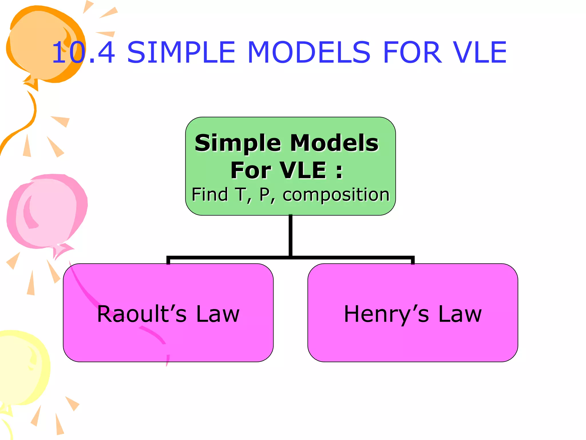
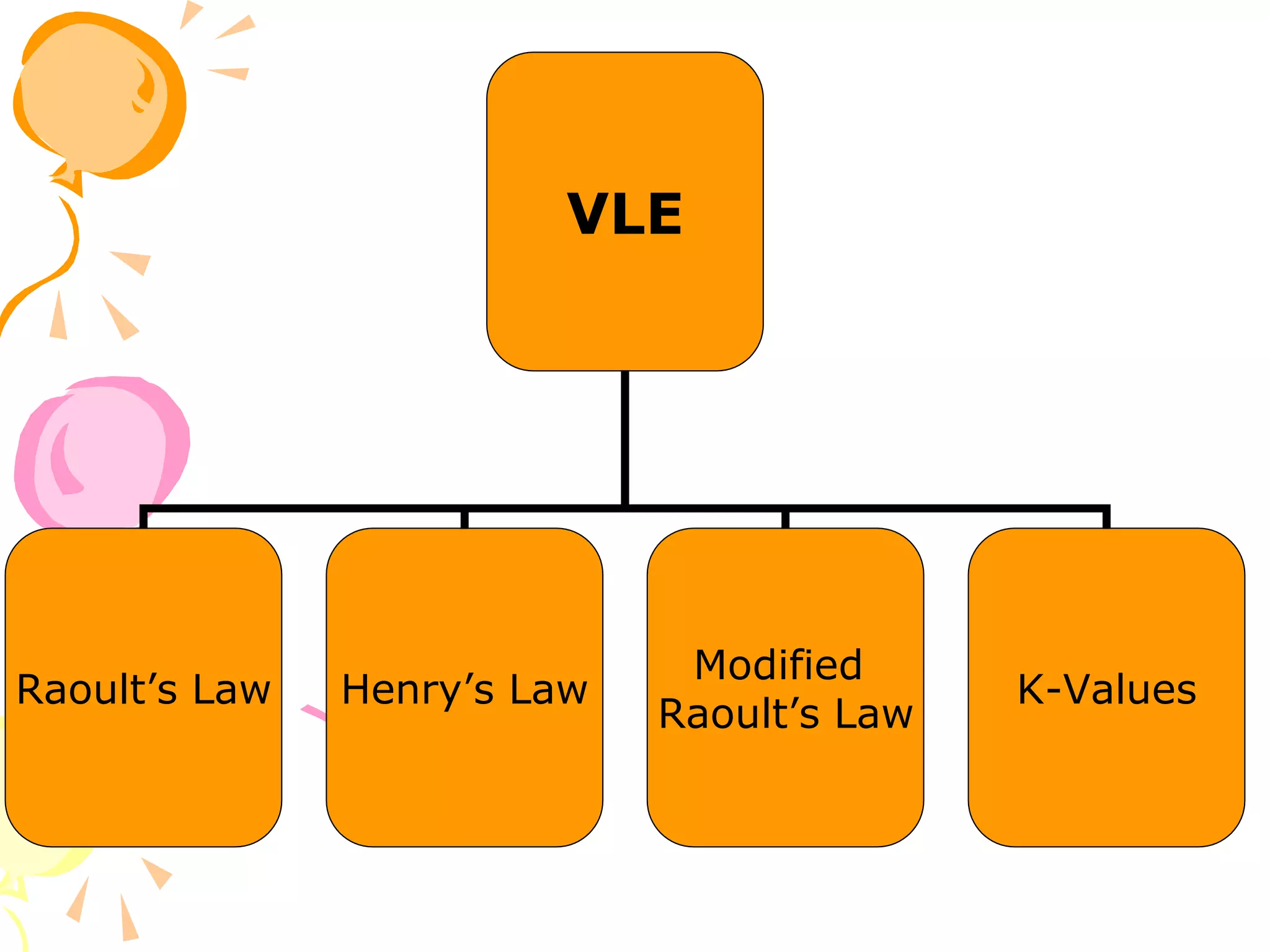
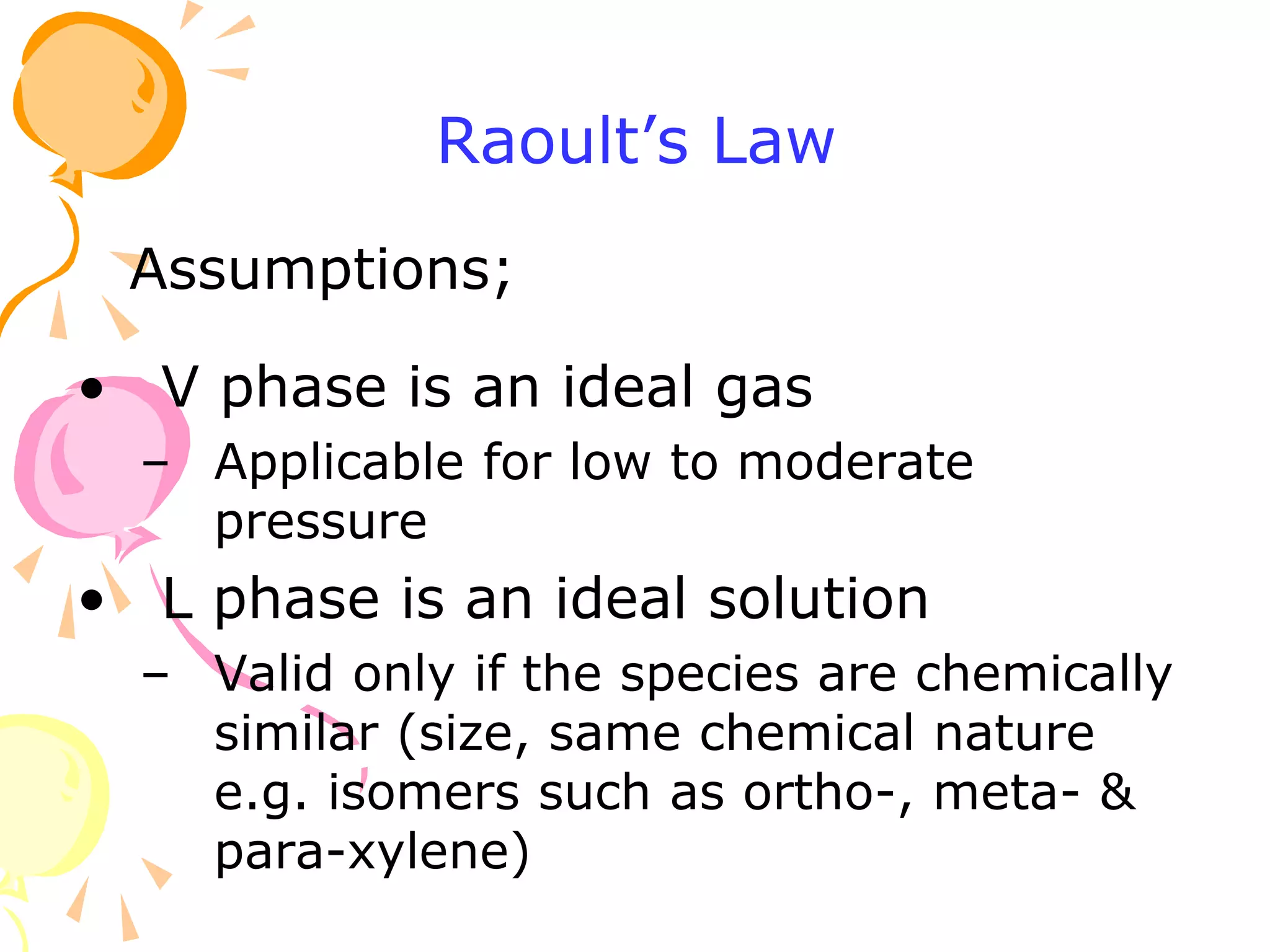
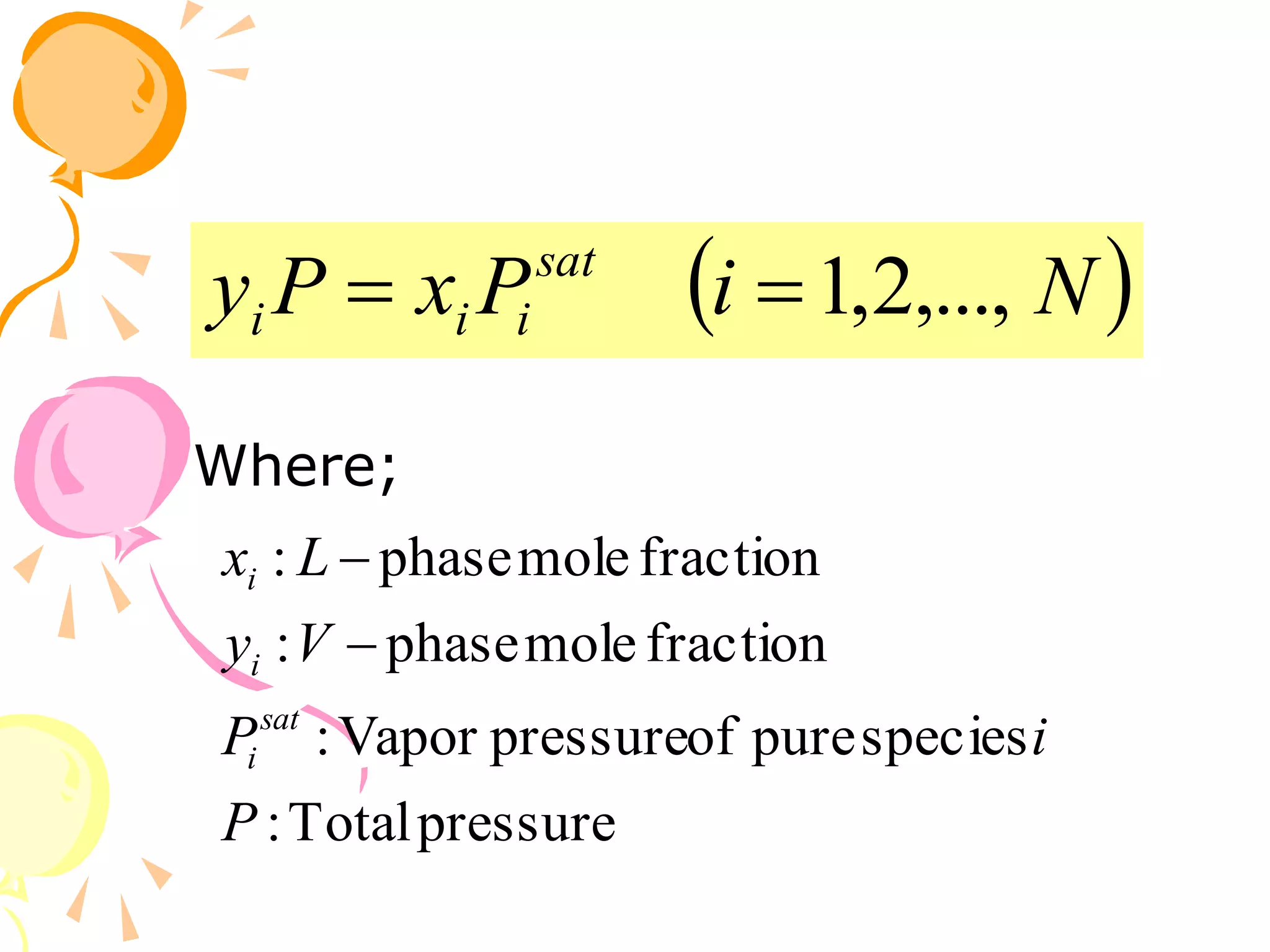
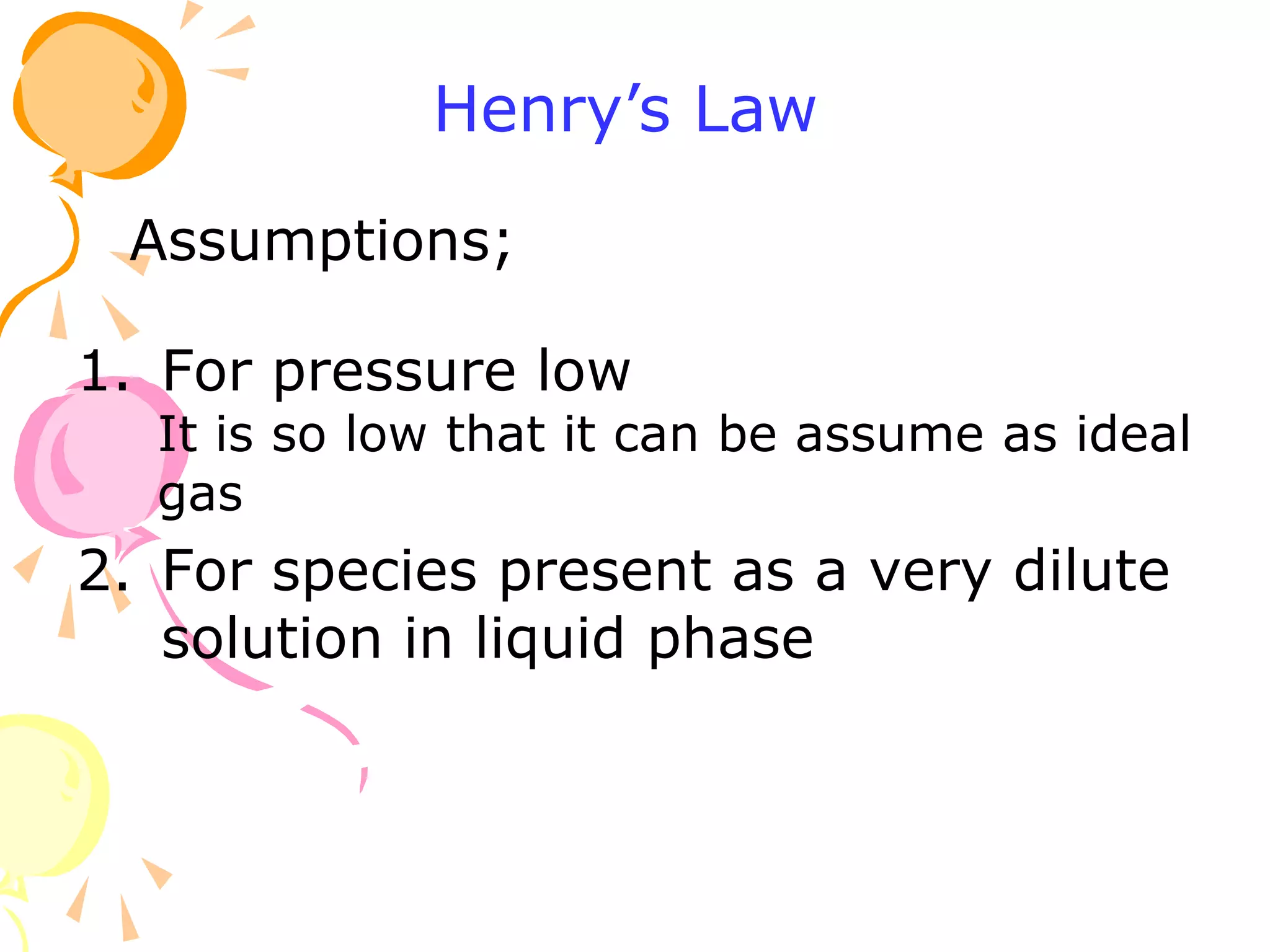
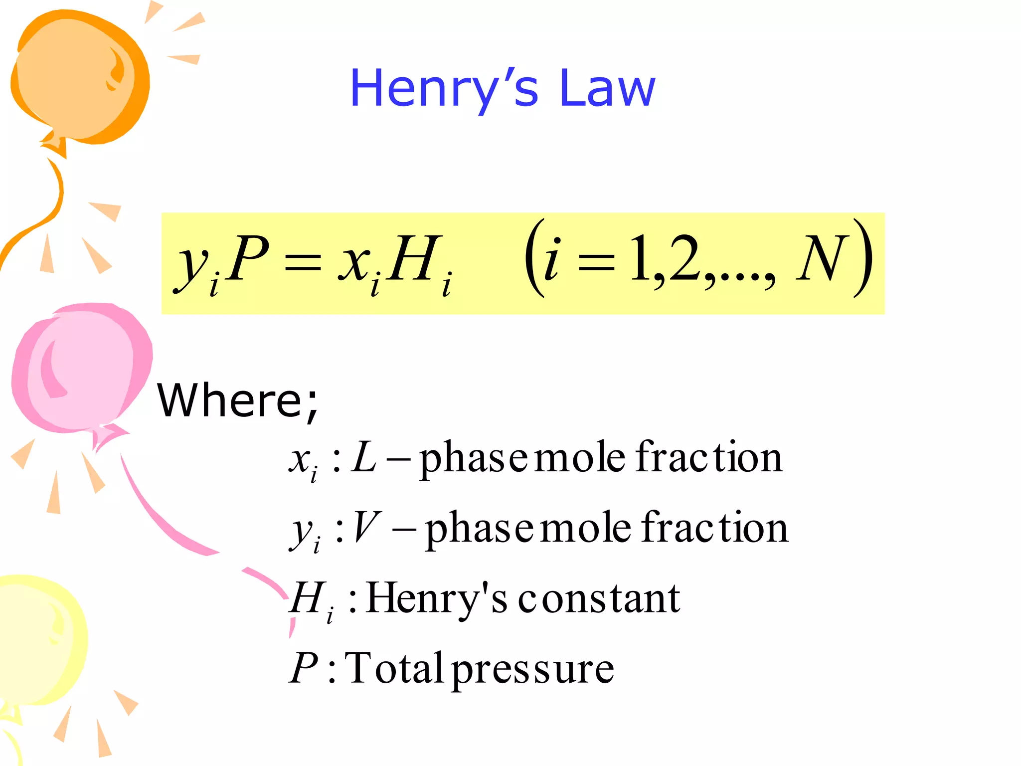
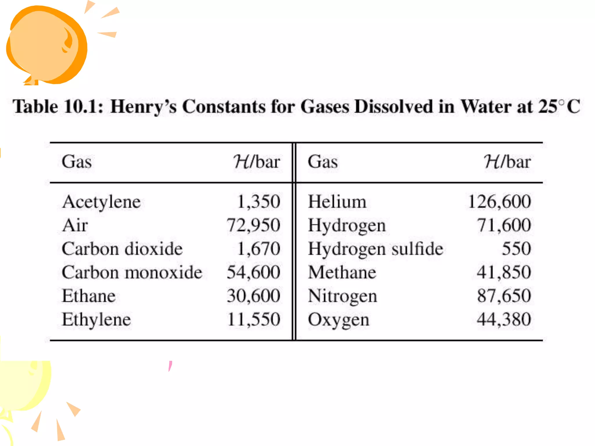
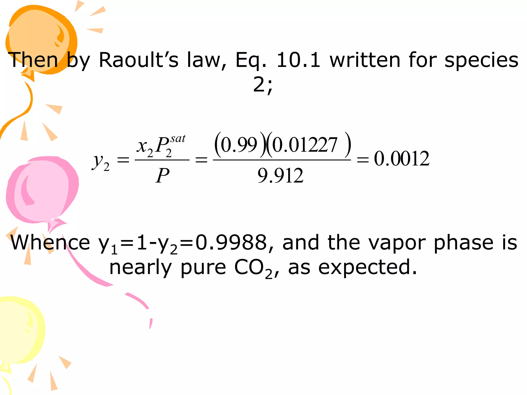
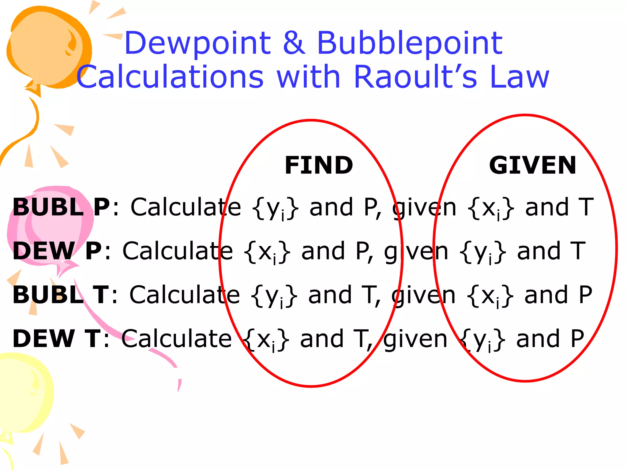
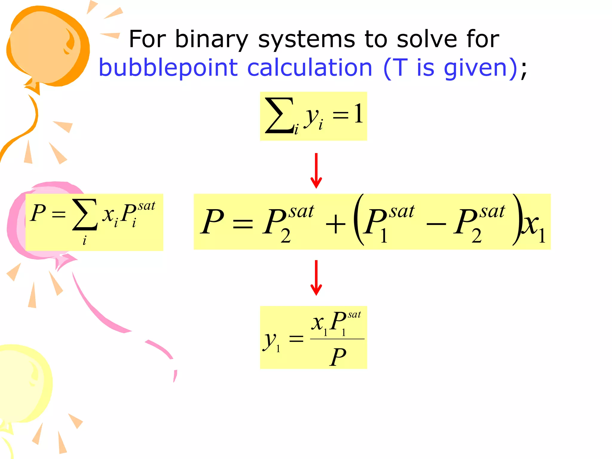
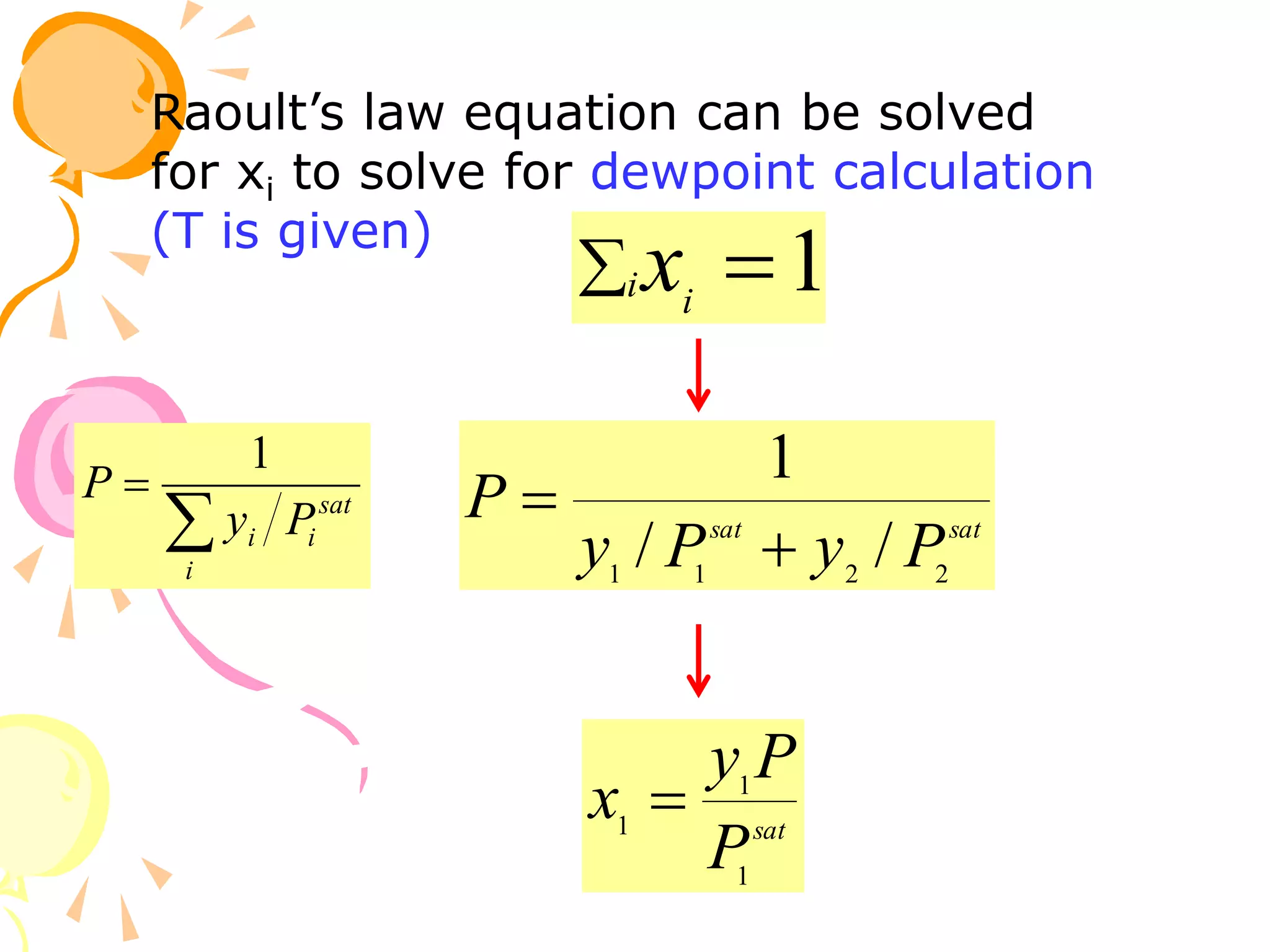
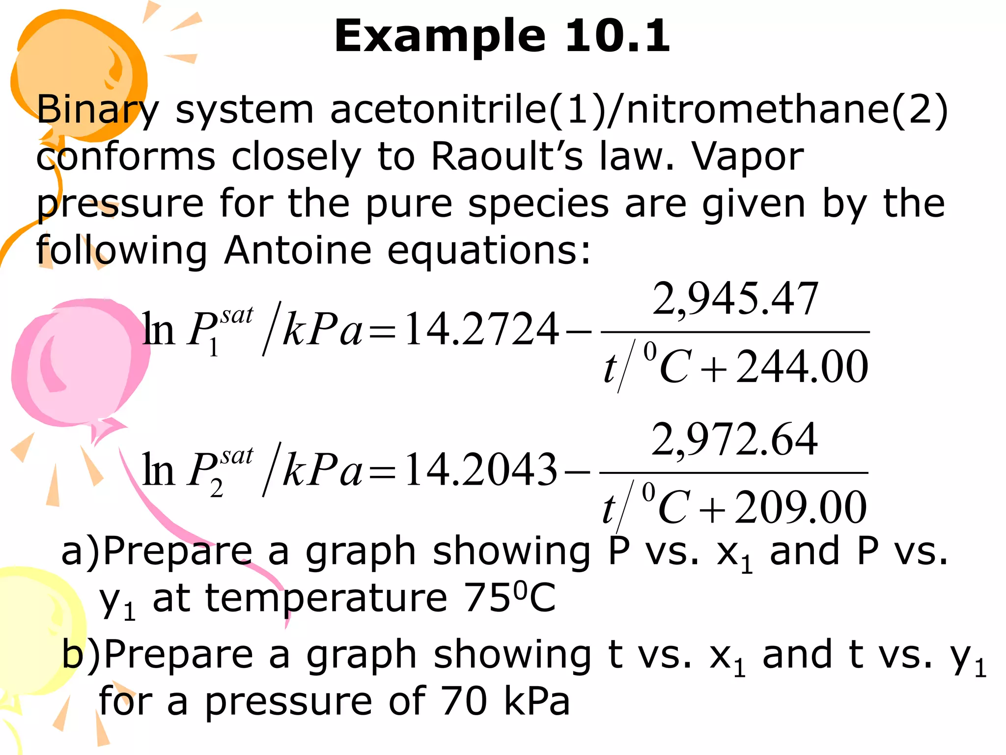
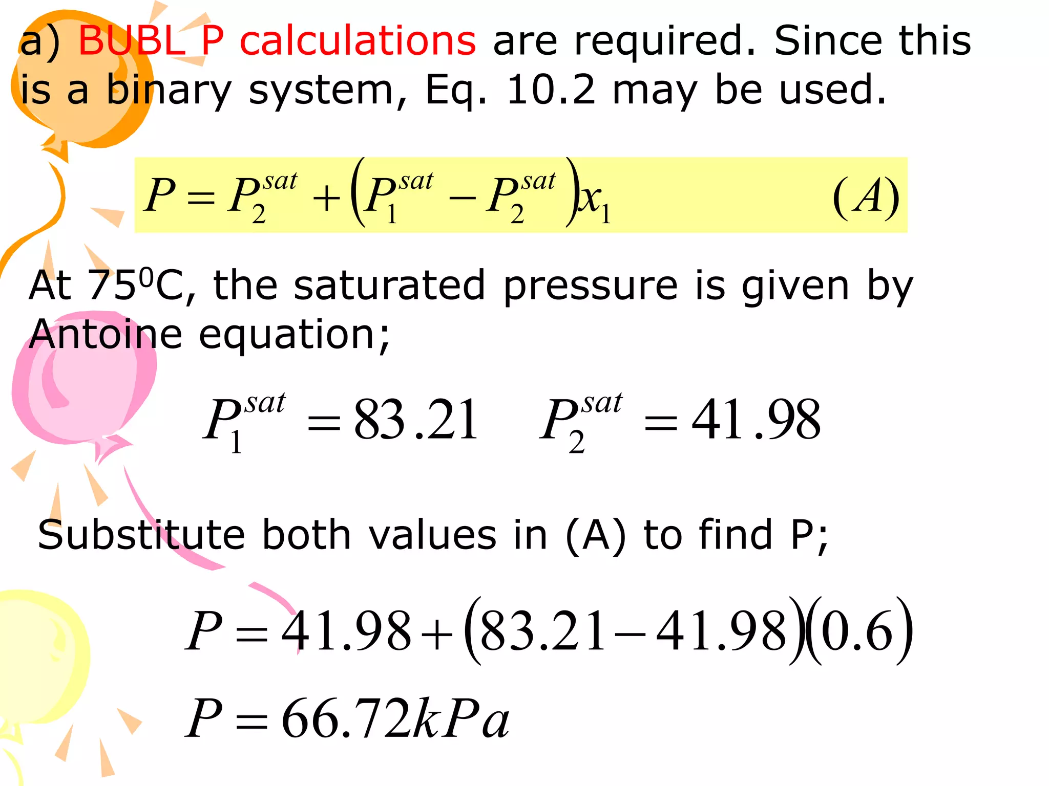
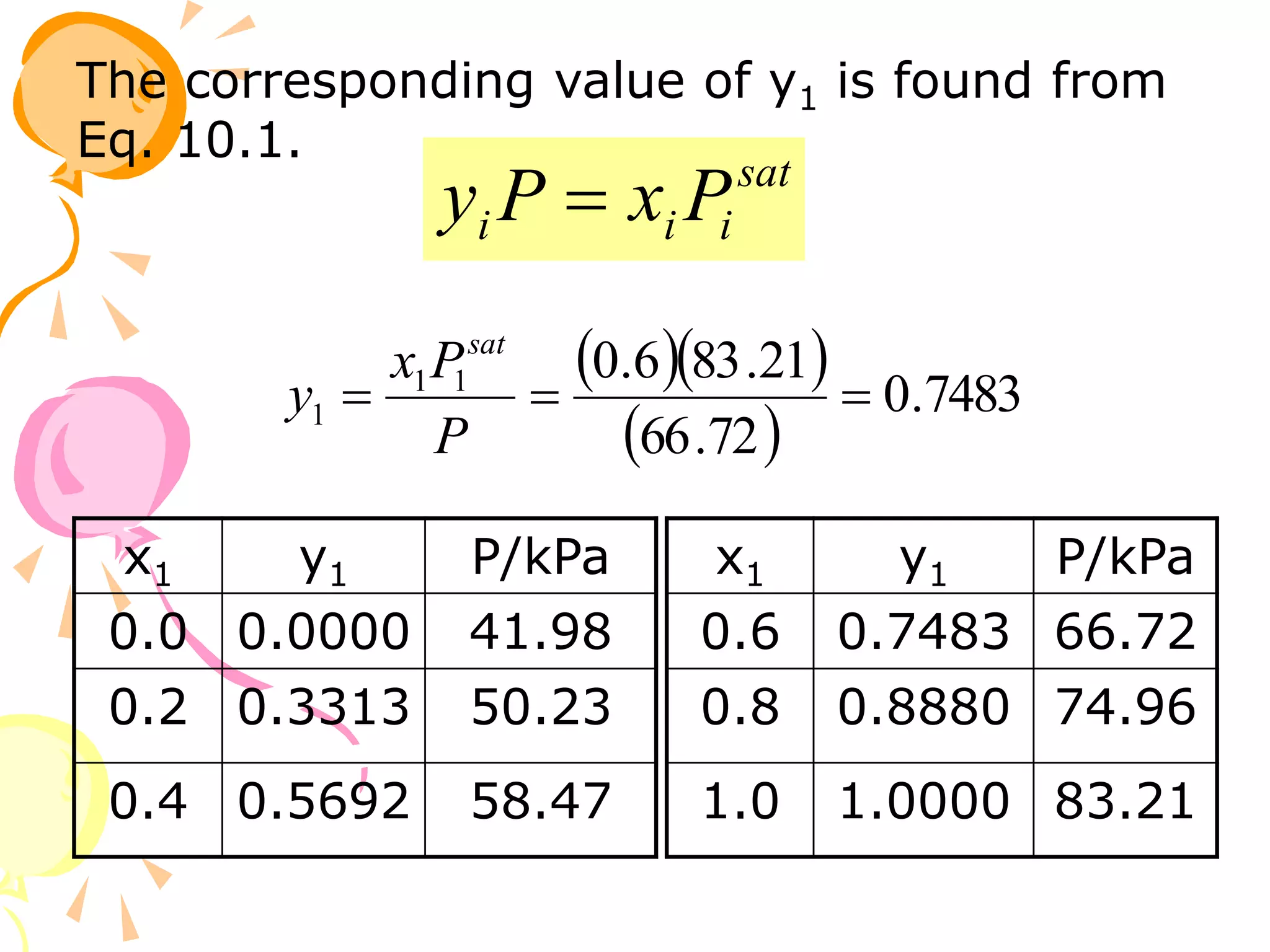
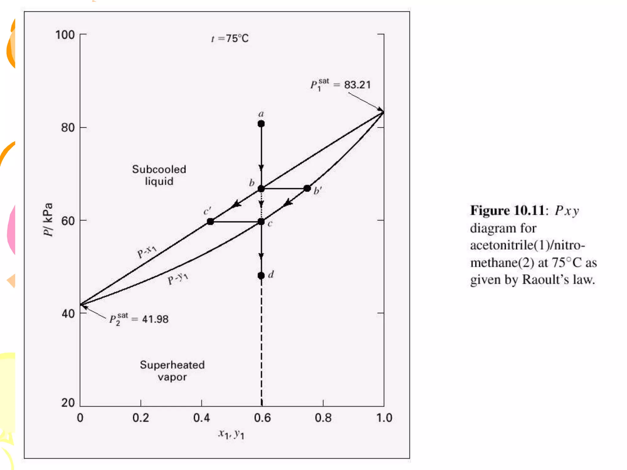
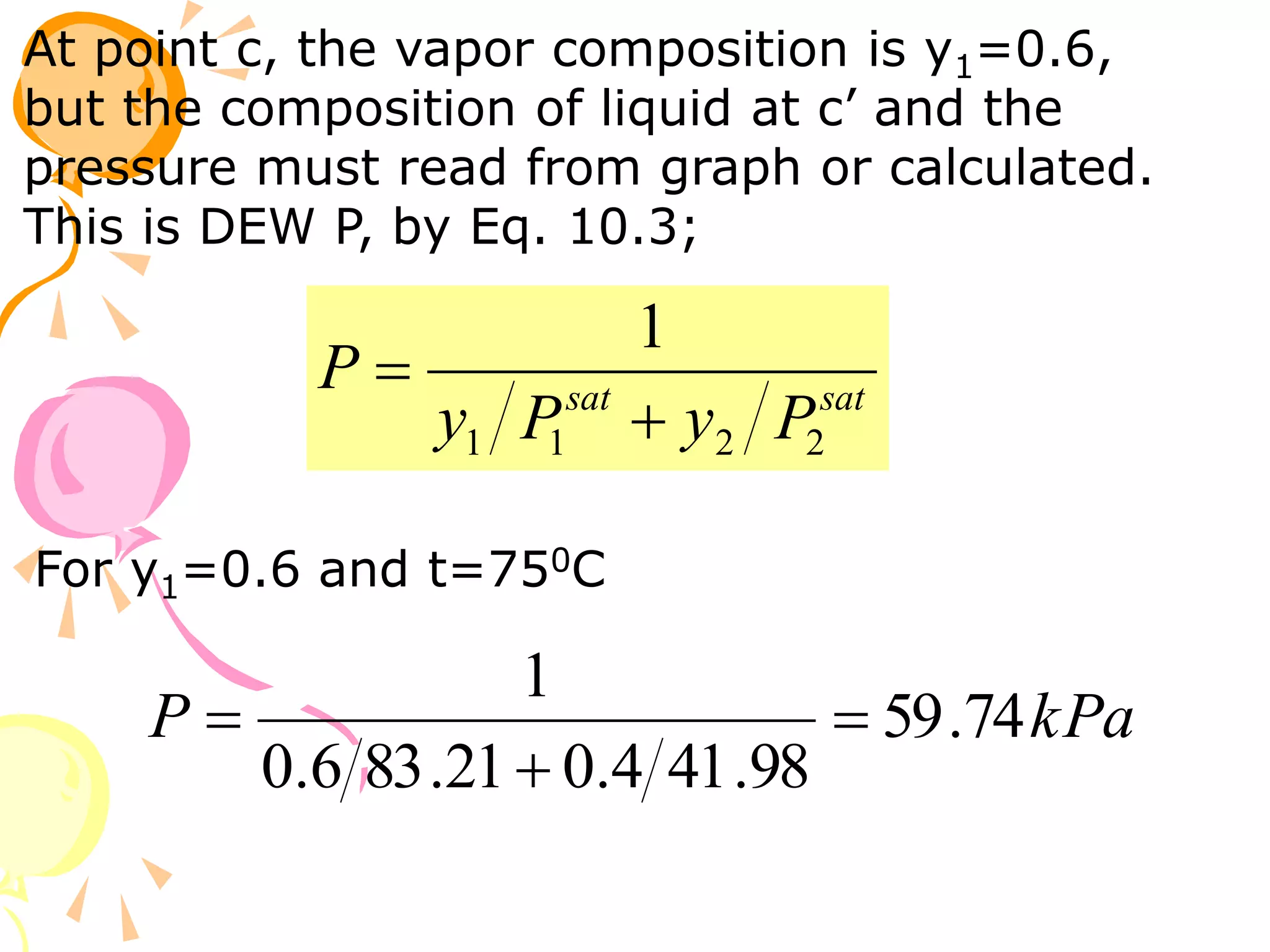
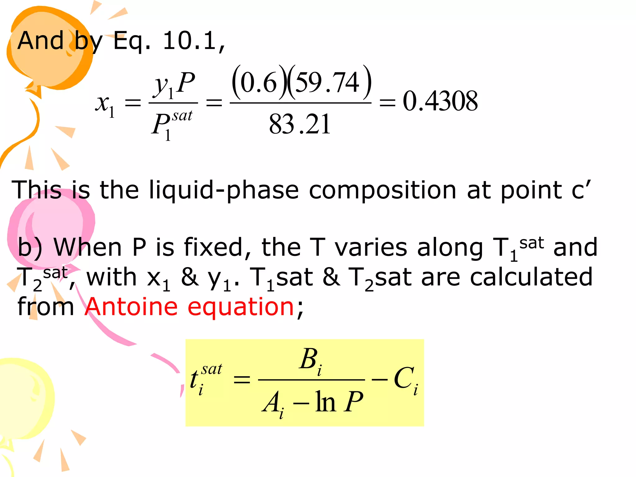
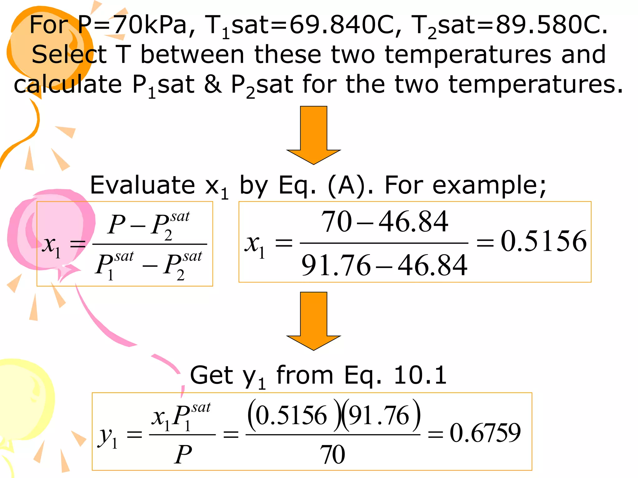
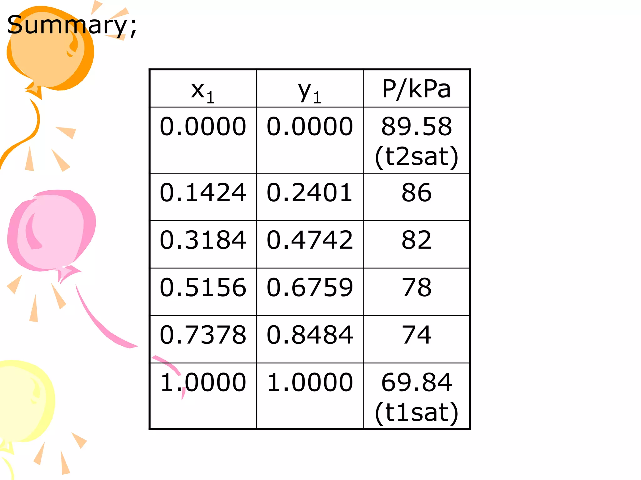
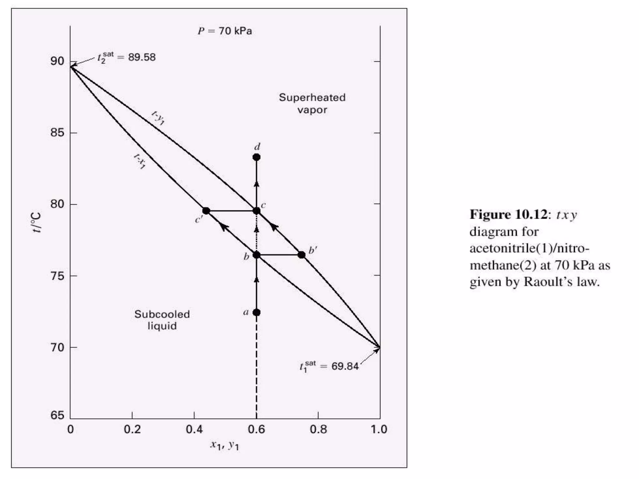
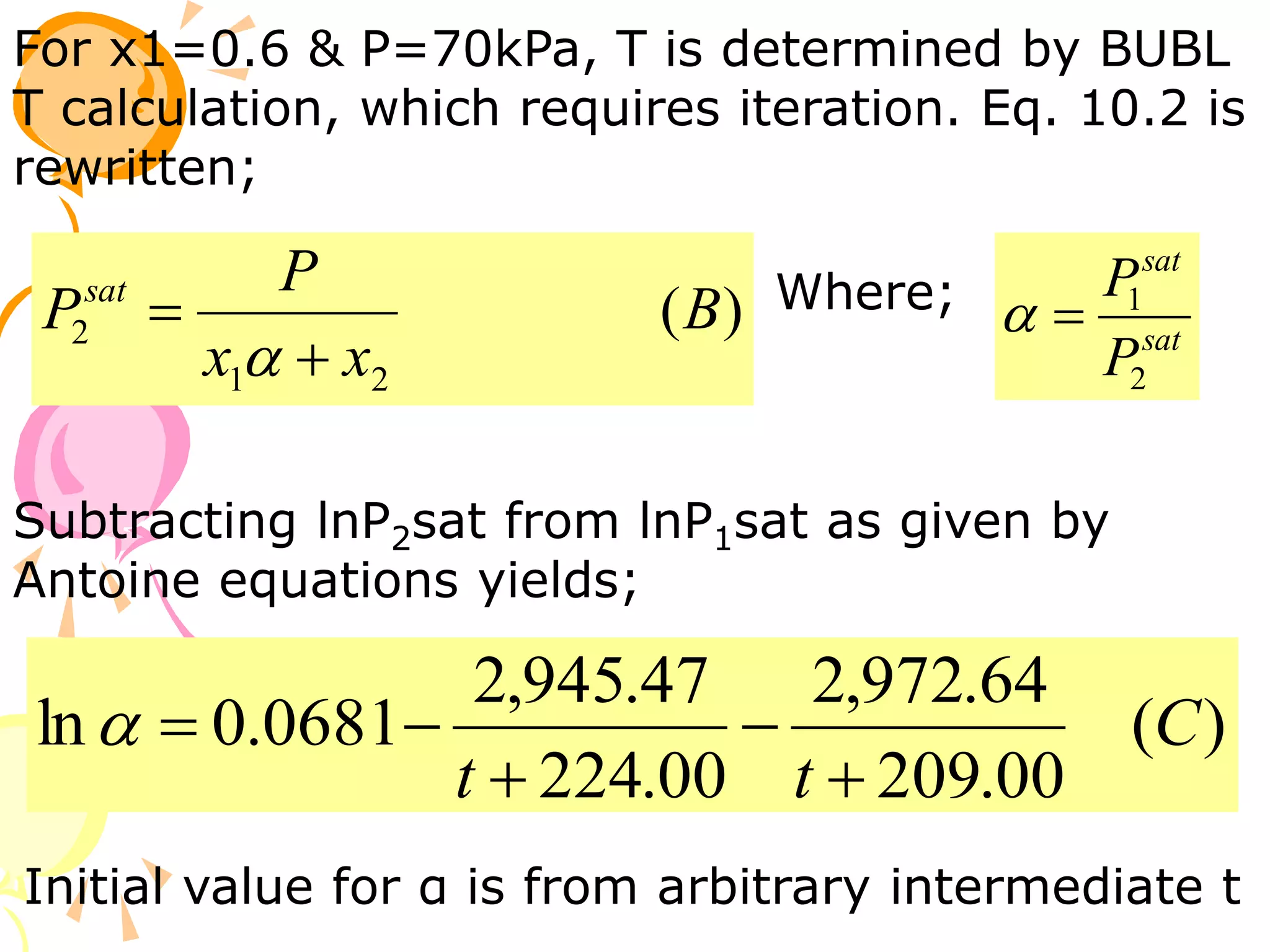
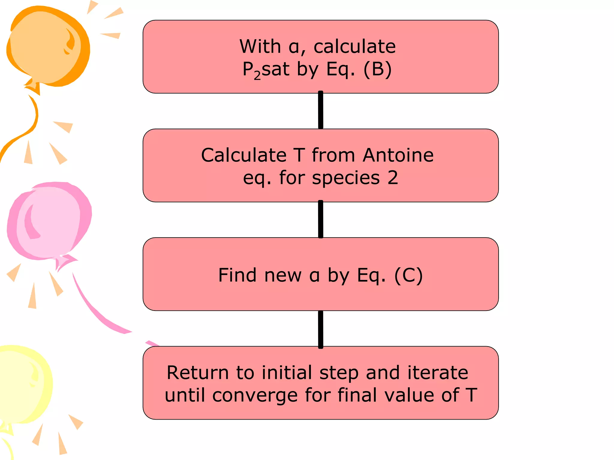
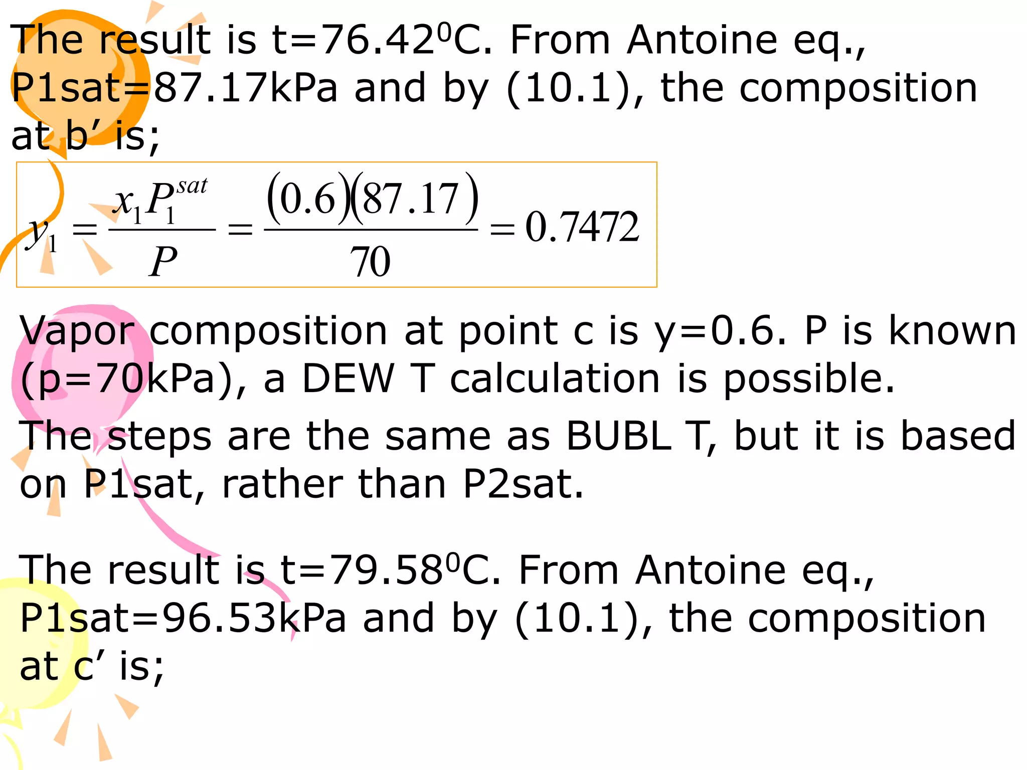
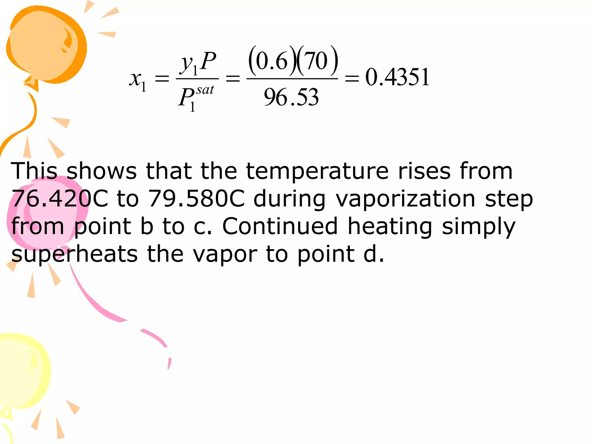
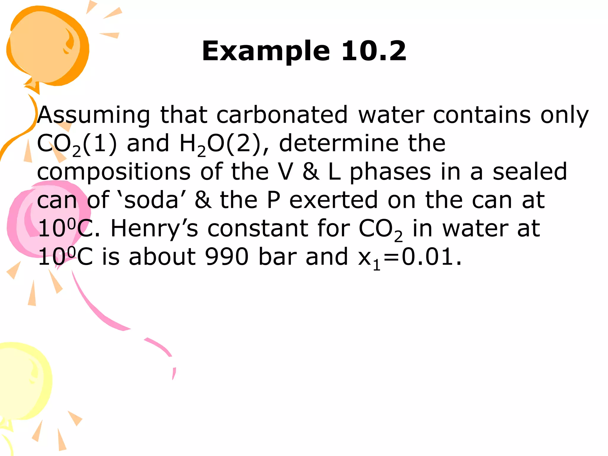
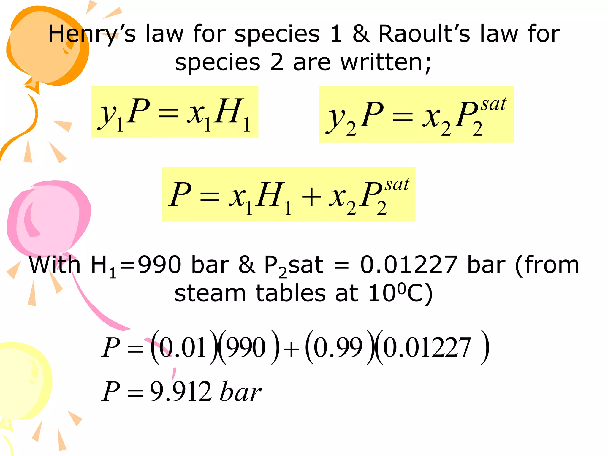
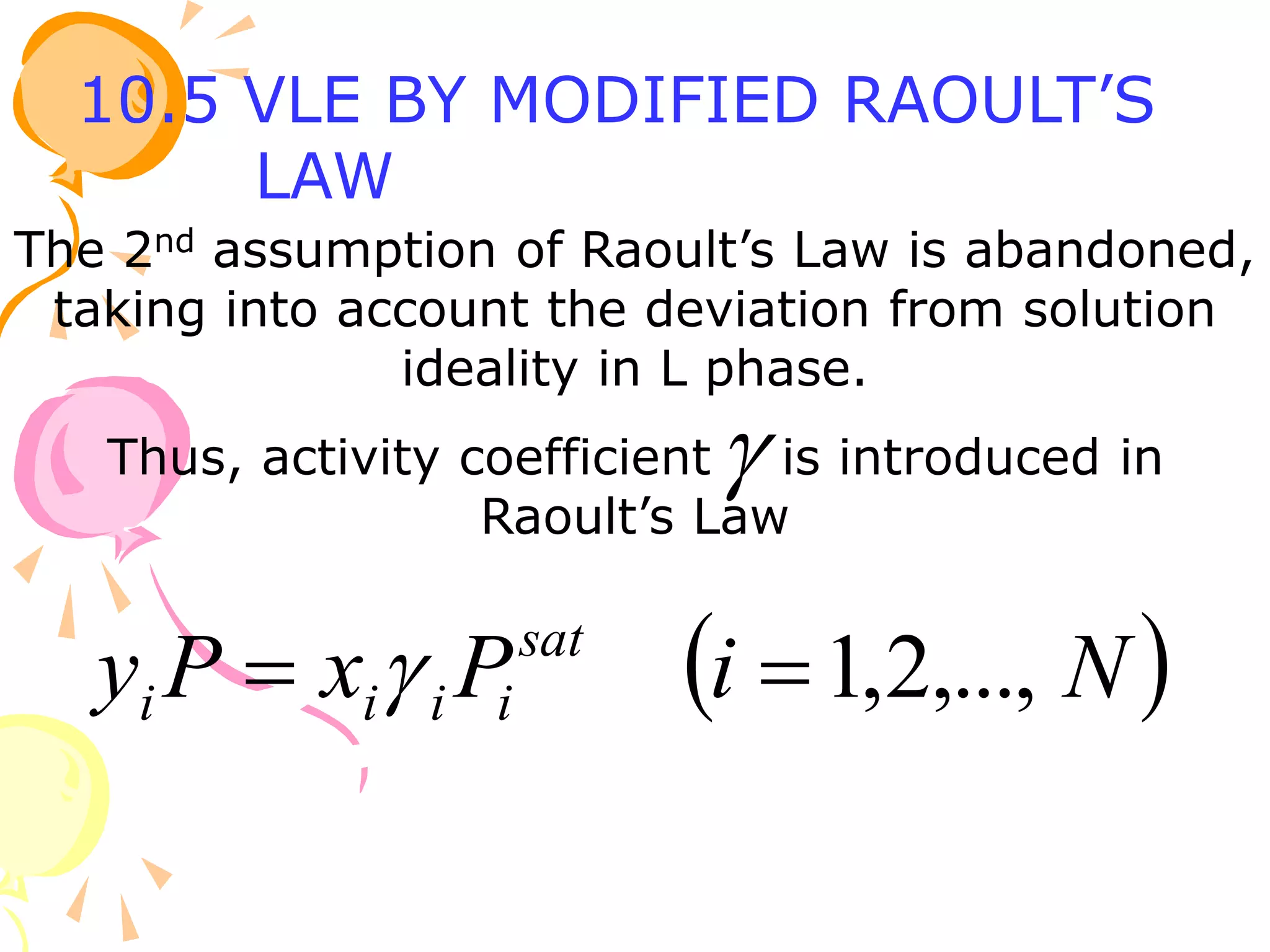
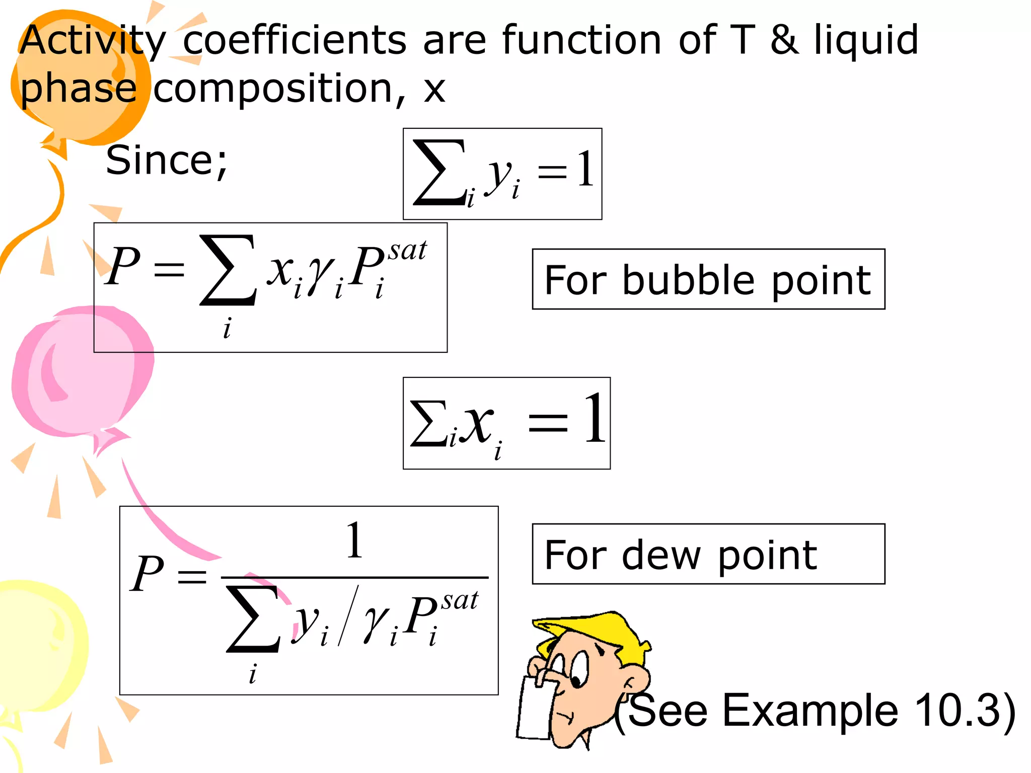
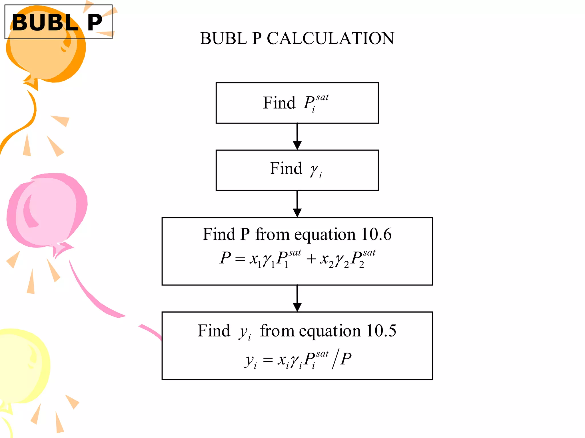
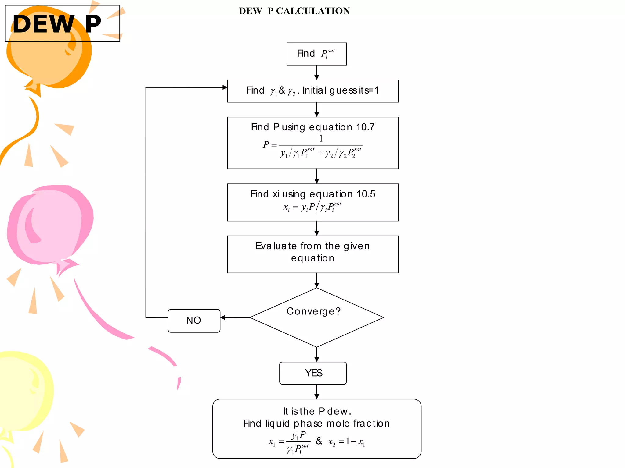
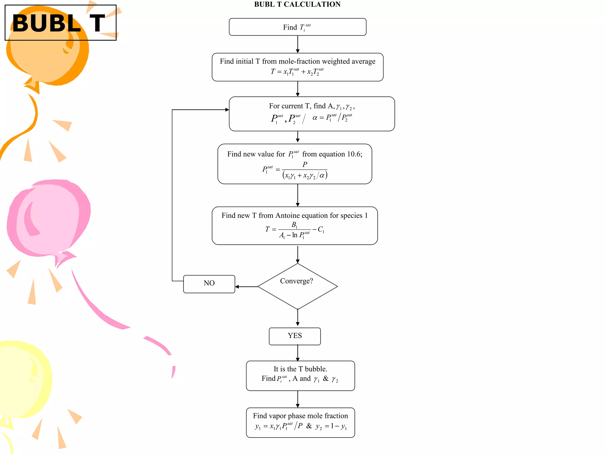
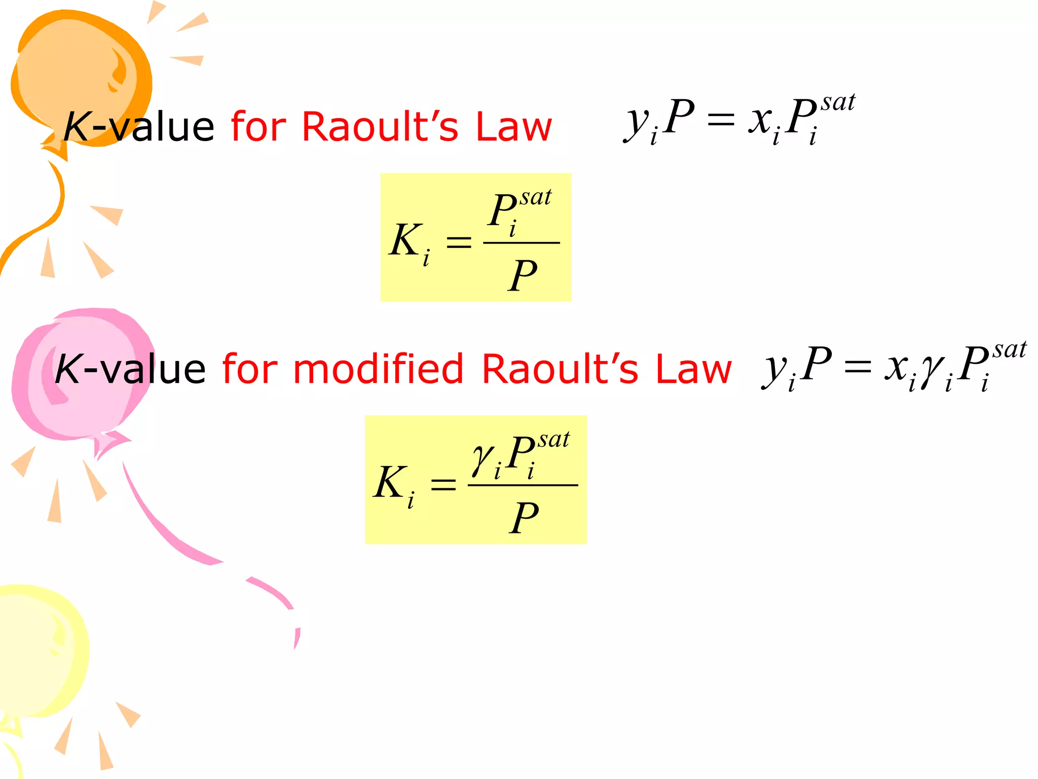
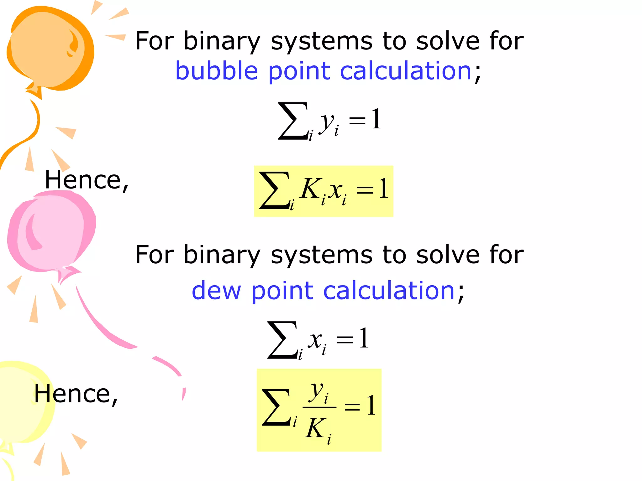
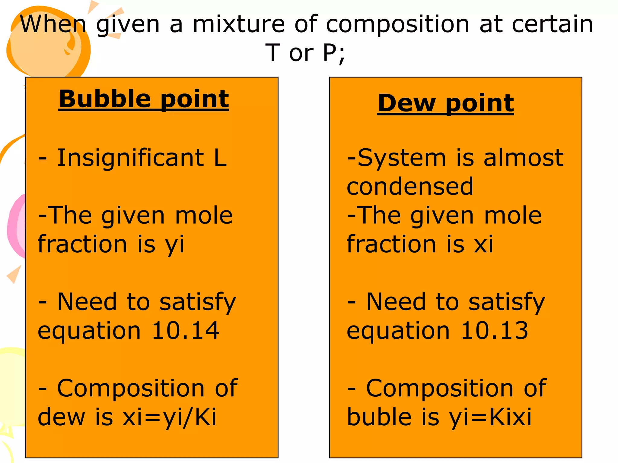
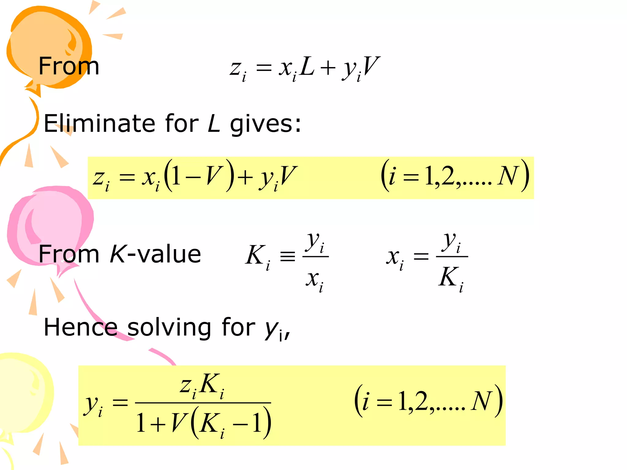
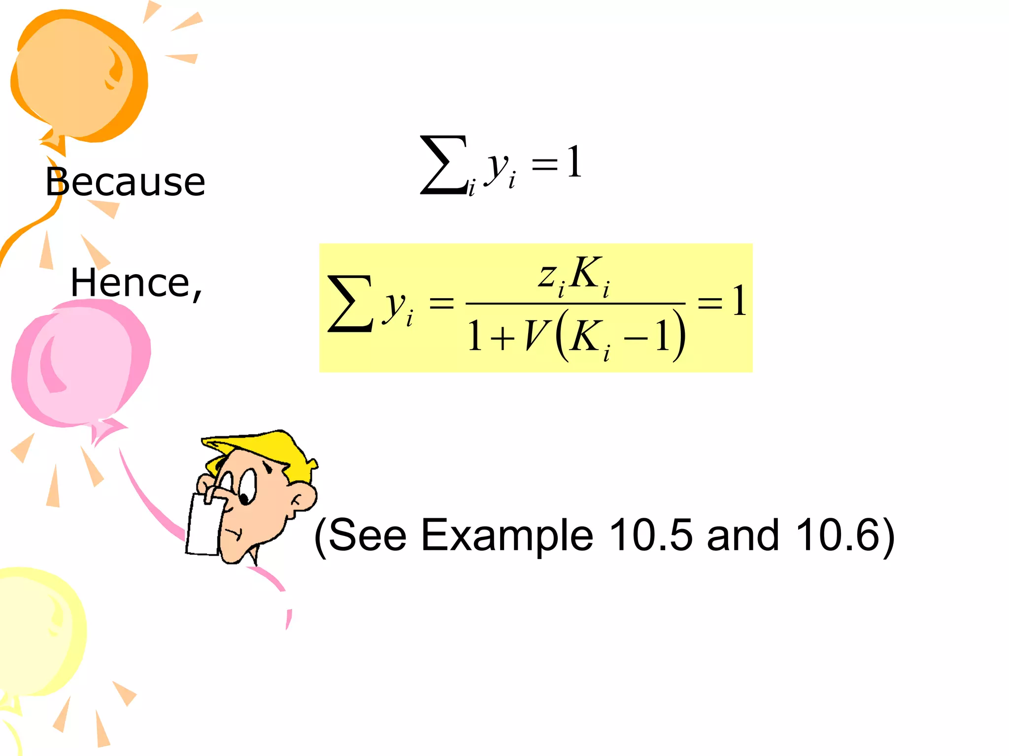
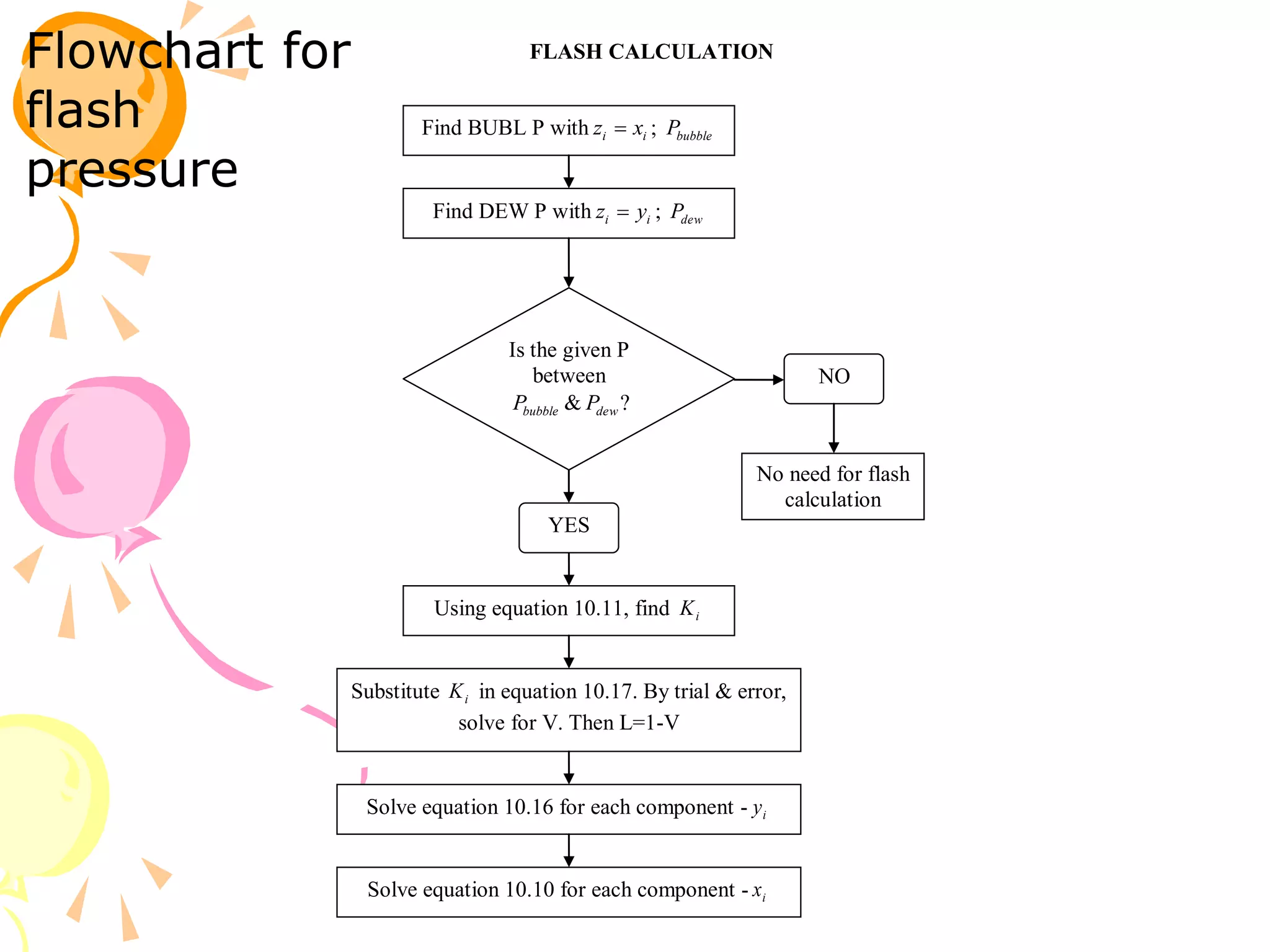
1. The document discusses vapor-liquid equilibrium (VLE) and some simple models for calculating VLE, including Raoult's law and Henry's law. 2. Raoult's law assumes an ideal gas in the vapor phase and an ideal solution in the liquid phase. Henry's law is applicable for very dilute solutions and low pressures where the vapor can be treated as an ideal gas. 3. Examples are provided to demonstrate calculating bubble point, dew point, and equilibrium conditions using these models. Modified Raoult's law is also introduced, which accounts for non-ideality in the liquid phase using activity coefficients.

1. Chapter 4
Chemical Engineering
Thermodynamics
VAPOR/LIQUID EQUILIBRIUM

2. • So far we have only dealt with pure
substances and constant composition
mixtures.
• We will move a step further where
the desired outcome is the
composition change.
• In system such as distillation &
absorption, if the system is not in
equilibrium, the mass transfer
between system will alter their
composition.

3. 10.1 Nature of Equilibrium
– Definition
– Measures of composition
10.2 The Phase Rule
– Duhem’s Theorem
10.3 VLE : Qualitative behavior
10.4 Simple Models for VLE
- Raoult’s Law
-Dewpoint & Bubblepoint Calculations with
Raoult’s Law
- Henry’s Law
Chapter Outline

4. 10.1 THE NATURE OF EQUILIBRIUM
Equilibrium : A static condition in
which no changes occur in the
macroscopic properties of a system with
time.
The T, P,
composition
reaches final
value which will
remain fixed:
equilibrium

5. Measure
of
composition
Mass or
mole fraction
Molar
concentration
Molar mass for
a mixture or
solution
m
m
m
m
x i
i
i




V
x
C i
i  

i
i
iM
x
M
Measures of composition

6. Equilibrium states are determined by;
–Phase Rule
–Duhem’s Theory
10.2 PHASE RULE & DUHEM’S
THEORY

7. Number of variables that may be
independently fixed in a system at equilibrium
=
Difference between total number of variables
that characterize the intensive state of the
system and number of independent equation
F = 2-π+N
Where : F – degrees of freedom
π – No of phase
N – No of species
The Phase Rule

8. For any closed system formed
initially from given masses of
prescribed chemical species, the
equilibrium state is completely
determined when any two (2)
independent variables are fixed
Duhem’s Theory

9. VLE: State of
coexistence of L
& V phases
Fig. 10.1 – Shows the P-T-
composition surfaces of
equilibrium states of
saturated V & saturated L
of a binary system
10.3 VLE: QUALITATIVE BEHAVIOR

10. • Under surface- sat. V states (P-T-y1)
• Upper surface- sat. L states (P-T-x1)
• Liquid at F, reduces pressure at
constant T & composition along FG,
the first bubble appear at L – bubble
point
• As pressure reduces, more & more L
vaporizes until completed at W; point
where last drop of L (dew) disappear
– dew point

13. Simple Models
For VLE :
Find T, P, composition
Raoult’s Law Henry’s Law
10.4 SIMPLE MODELS FOR VLE

14. Raoult’s Law
• V phase is an ideal gas
– Applicable for low to moderate
pressure
• L phase is an ideal solution
– Valid only if the species are chemically
similar (size, same chemical nature
e.g. isomers such as ortho-, meta- &
para-xylene)
Assumptions;

15.  
N
i
P
x
P
y sat
i
i
i ,...,
2
,
1


Where;
pressure
Total
:
species
pure
of
pressure
Vapor
:
fraction
mole
phase
:
fraction
mole
phase
:
P
i
P
V
y
L
x
sat
i
i
i



16. BUBL P: Calculate {yi} and P, given {xi} and T
DEW P: Calculate {xi} and P, given {yi} and T
BUBL T: Calculate {yi} and T, given {xi} and P
DEW T: Calculate {xi} and T, given {yi} and P
Dewpoint & Bubblepoint
Calculations with Raoult’s Law
FIND GIVEN

17. For binary systems to solve for
bubblepoint calculation (T is given);
1

i i
y


i
sat
i
i P
x
P   1
2
1
2 x
P
P
P
P sat
sat
sat



P
P
x
y
sat
1
1
1


18. 

i
sat
i
i P
y
P
1
Raoult’s law equation can be solved
for xi to solve for dewpoint calculation
(T is given)
1

i i
x
sat
sat
P
y
P
y
P
2
2
1
1
/
/
1


sat
P
P
y
x
1
1
1


19. Example 10.1
Binary system acetonitrile(1)/nitromethane(2)
conforms closely to Raoult’s law. Vapor
pressure for the pure species are given by the
following Antoine equations:
00
.
209
64
.
972
,
2
2043
.
14
ln
00
.
244
47
.
945
,
2
2724
.
14
ln
0
2
0
1






C
t
kPa
P
C
t
kPa
P
sat
sat
a)Prepare a graph showing P vs. x1 and P vs.
y1 at temperature 750C
b)Prepare a graph showing t vs. x1 and t vs. y1
for a pressure of 70 kPa

20. a) BUBL P calculations are required. Since this
is a binary system, Eq. 10.2 may be used.
  )
(
1
2
1
2 A
x
P
P
P
P sat
sat
sat



At 750C, the saturated pressure is given by
Antoine equation;
98
.
41
21
.
83 2
1 
 sat
sat
P
P
Substitute both values in (A) to find P;
  
kPa
P
P
72
.
66
6
.
0
98
.
41
21
.
83
98
.
41





21. The corresponding value of y1 is found from
Eq. 10.1.
sat
i
i
i P
x
P
y 
x1 y1 P/kPa
0.0 0.0000 41.98
0.2 0.3313 50.23
0.4 0.5692 58.47
x1 y1 P/kPa
0.6 0.7483 66.72
0.8 0.8880 74.96
1.0 1.0000 83.21
  
 
7483
.
0
72
.
66
21
.
83
6
.
0
1
1
1 


P
P
x
y
sat

23. At point c, the vapor composition is y1=0.6,
but the composition of liquid at c’ and the
pressure must read from graph or calculated.
This is DEW P, by Eq. 10.3;
sat
sat
P
y
P
y
P
2
2
1
1
1


For y1=0.6 and t=750C
kPa
P 74
.
59
98
.
41
4
.
0
21
.
83
6
.
0
1




24. And by Eq. 10.1,
   4308
.
0
21
.
83
74
.
59
6
.
0
1
1
1 

 sat
P
P
y
x
This is the liquid-phase composition at point c’
b) When P is fixed, the T varies along T1
sat and
T2
sat, with x1 & y1. T1sat & T2sat are calculated
from Antoine equation;
i
i
i
sat
i C
P
A
B
t 


ln

25. For P=70kPa, T1sat=69.840C, T2sat=89.580C.
Select T between these two temperatures and
calculate P1sat & P2sat for the two temperatures.
Evaluate x1 by Eq. (A). For example;
sat
sat
sat
P
P
P
P
x
2
1
2
1


 5156
.
0
84
.
46
76
.
91
84
.
46
70
1 



x
Get y1 from Eq. 10.1
   6759
.
0
70
76
.
91
5156
.
0
1
1
1 


P
P
x
y
sat

26. Summary;
x1 y1 P/kPa
0.0000 0.0000 89.58
(t2sat)
0.1424 0.2401 86
0.3184 0.4742 82
0.5156 0.6759 78
0.7378 0.8484 74
1.0000 1.0000 69.84
(t1sat)

28. For x1=0.6 & P=70kPa, T is determined by BUBL
T calculation, which requires iteration. Eq. 10.2 is
rewritten;
)
(
2
1
2 B
x
x
P
Psat


 sat
sat
P
P
2
1


Where;
Subtracting lnP2sat from lnP1sat as given by
Antoine equations yields;
)
(
00
.
209
64
.
972
,
2
00
.
224
47
.
945
,
2
0681
.
0
ln C
t
t 





Initial value for α is from arbitrary intermediate t

29. With α, calculate
P2sat by Eq. (B)
Calculate T from Antoine
eq. for species 2
Find new α by Eq. (C)
Return to initial step and iterate
until converge for final value of T

30. The result is t=76.420C. From Antoine eq.,
P1sat=87.17kPa and by (10.1), the composition
at b’ is;
   7472
.
0
70
17
.
87
6
.
0
1
1
1 


P
P
x
y
sat
Vapor composition at point c is y=0.6. P is known
(p=70kPa), a DEW T calculation is possible.
The steps are the same as BUBL T, but it is based
on P1sat, rather than P2sat.
The result is t=79.580C. From Antoine eq.,
P1sat=96.53kPa and by (10.1), the composition
at c’ is;

31.    4351
.
0
53
.
96
70
6
.
0
1
1
1 

 sat
P
P
y
x
This shows that the temperature rises from
76.420C to 79.580C during vaporization step
from point b to c. Continued heating simply
superheats the vapor to point d.

32. 1. For pressure low
It is so low that it can be assume as ideal
gas
2. For species present as a very dilute
solution in liquid phase
Assumptions;
Henry’s Law

33.  
N
i
H
x
P
y i
i
i ,...,
2
,
1


Where;
pressure
Total
:
constant
s
Henry'
:
fraction
mole
phase
:
fraction
mole
phase
:
P
H
V
y
L
x
i
i
i


Henry’s Law

35. Example 10.2
Assuming that carbonated water contains only
CO2(1) and H2O(2), determine the
compositions of the V & L phases in a sealed
can of ‘soda’ & the P exerted on the can at
100C. Henry’s constant for CO2 in water at
100C is about 990 bar and x1=0.01.

36. Henry’s law for species 1 & Raoult’s law for
species 2 are written;
1
1
1 H
x
P
y  sat
P
x
P
y 2
2
2 
With H1=990 bar & P2sat = 0.01227 bar (from
steam tables at 100C)
     
bar
P
P
912
.
9
01227
.
0
99
.
0
990
01
.
0



sat
P
x
H
x
P 2
2
1
1 


37. Then by Raoult’s law, Eq. 10.1 written for species
2;
   0012
.
0
912
.
9
01227
.
0
99
.
0
2
2
2 


P
P
x
y
sat
Whence y1=1-y2=0.9988, and the vapor phase is
nearly pure CO2, as expected.

38. Review
• What is bubble point?
• What is dew point?
• We have previously go through the 2
simplest models for solving VLE
problems
– Raoult’s Law
– Henry’s Law

39. Chapter Outline
10.5 VLE by modified Raoult’s law
10.6 VLE from K-value correlations
- Flash calculation

40. VLE
Raoult’s Law Henry’s Law
Modified
Raoult’s Law
K-Values

41. The 2nd assumption of Raoult’s Law is abandoned,
taking into account the deviation from solution
ideality in L phase.
Thus, activity coefficient is introduced in
Raoult’s Law

 
N
i
P
x
P
y sat
i
i
i
i ,...,
2
,
1

 
10.5 VLE BY MODIFIED RAOULT’S
LAW

42. Activity coefficients are function of T & liquid
phase composition, x
1

i i
y


i
sat
i
i
i P
x
P 


i
sat
i
i
i P
y
P

1
For bubble point
For dew point
Since;
(See Example 10.3)
1

i i
x

43. BUBL P
BUBL P CALCULATION
Find sat
i
P
Find i

Find P from equation 10.6
sat
sat
P
x
P
x
P 2
2
2
1
1
1 
 

Find i
y from equation 10.5
P
P
x
y sat
i
i
i
i 


44. DEW P
DEW P CALCULATION
Find sat
i
P
Find 1
 & 2
 . Initial guess its=1
Find P using equation 10.7
sat
sat
P
y
P
y
P
2
2
2
1
1
1
1

 

Find xi using equation 10.5
sat
i
i
i
i P
P
y
x 

Evaluate from the given
equation
Converge?
NO
YES
It is the P dew.
Find liquid phase mole fraction
sat
P
P
y
x
1
1
1
1

 & 1
2 1 x
x 


45. BUBL T
BUBL T CALCULATION
Find initial T from mole-fraction weighted average
sat
sat
T
x
T
x
T 2
2
1
1 

Find sat
i
T
For current T, find A, 1
 , 2
 ,
sat
sat
P
P 2
1
,
sat
sat
P
P 2
1


Find new value for sat
P1 from equation 10.6;
 


 2
2
1
1
1
x
x
P
Psat


Find new T from Antoine equation for species 1
1
1
1
1
ln
C
P
A
B
T sat



Converge?
NO
YES
It is the T bubble.
Find sat
i
P , A and 1
 & 2

Find vapor phase mole fraction
P
P
x
y sat
1
1
1
1 
 & 1
2 1 y
y 


46. DEW T
DEW T CALCULATION
Find initial T from mole-fraction weighted average
sat
sat
T
y
T
y
T 2
2
1
1 

Find sat
i
T
For current T, find A, sat
sat
P
P 2
1 ,
sat
sat
P
P 2
1


Find new value for sat
P1 from equation 10.7;









 

 2
2
1
1
1
y
y
P
Psat
Find new T from Antoine equation for species 1
1
1
1
1
ln
C
P
A
B
T sat



Converge?
NO
YES
It is the T bubble.
Find sat
i
P , A and 1
 & 2

Find vapor phase mole fraction
P
P
x
y sat
1
1
1
1 
 & 1
2 1 y
y 

Find sat
P
P
y
x 1
1
1
1 
 & 1
2 1 x
x 

Calculate 2
1 &
 from given correlation

47. AZEOTROPE
When x1=y1, the dew
point and bubble point
curves are tangent to
the same horizontal line
A boiling L of this
composition produce a
vapor exactly the same
composition; L does not
change in composition
as it evaporates

48. )
8
.
10
(
2
2
1
1
12
x
y
x
y


Relative volatility;
  sat
sat
x
P
A
P
2
1
0
12
exp
1



 
A
P
P
sat
sat
x
exp
2
1
1
12 1



If one limit is >1 &
the other limit is
<1; azeotrope
exists.

49. 10.6 VLE FROM K-VALUE
CORRELATTIONS
The partition between liquid and vapor
phases of a chemical species is equilibrium
ratio, Ki.
i
i
i
x
y
K 
This quantity is called K-value.

50. sat
i
i
i P
x
P
y 
K-value for Raoult’s Law
P
P
K
sat
i
i 
K-value for modified Raoult’s Law
sat
i
i
i
i P
x
P
y 

P
P
K
sat
i
i
i



51. Hence,
For binary systems to solve for
bubble point calculation;
1

i i
y
1

 i
i i x
K
For binary systems to solve for
dew point calculation;
1

i i
x
Hence, 1

i
i
i
K
y

52. K-value
from
DePriester
chart
-Low T
range

53. K-value
from
DePriester
chart
-High T
range

54. When given a mixture of composition at certain
T or P;
Bubble point
- Insignificant L
-The given mole
fraction is yi
- Need to satisfy
equation 10.14
- Composition of
dew is xi=yi/Ki
Dew point
-System is almost
condensed
-The given mole
fraction is xi
- Need to satisfy
equation 10.13
- Composition of
buble is yi=Kixi

55. Flash Calculation
The most important application of VLE.
Originates from a fact that a liquid at a
pressure equal to or greater that its
bubble point pressure ‘flashes’ or
evaporates when the pressure is
reduced, producing a two-phase system
of vapor and liquid in equilibrium.

56. FLASH CALCULATION
V
L
Feed, F
Vapor, V
Liquid, L
Liquid at P > Pbubble
partially evaporates
when P is reduced,
producing 2-phase
system of V & L in
equilibrium
Find; T, P, z

57. In a system with one mole chemical
species with an overall composition by
set of mole fraction, zi.
Li would be the moles of liquid with mol
fraction xi and V be the moles of vapor
with the mol fraction of yi:
1

V
L
z
 
N
i
V
y
L
x
z i
i
i ,.....
2
,
1




58. V
y
L
x
z i
i
i 

From
Eliminate for L gives:
   
N
i
V
y
V
x
z i
i
i ,.....
2
,
1
1 



i
i
i
x
y
K 
From K-value
i
i
i
K
y
x 
Hence solving for yi,
 
 
N
i
K
V
K
z
y
i
i
i
i ,.....
2
,
1
1
1





59. Hence,
1

i i
y
 
1
1
1





i
i
i
i
K
V
K
z
y
(See Example 10.5 and 10.6)
Because

60. FLASH CALCULATION
Find BUBL P with i
i x
z  ; bubble
P
Find DEW P with i
i y
z  ; dew
P
Using equation 10.11, find i
K
Is the given P
between
dew
bubble P
P & ?
NO
No need for flash
calculation
YES
Substitute i
K in equation 10.17. By trial & error,
solve for V. Then L=1-V
Solve equation 10.16 for each component - i
y
Solve equation 10.10 for each component - i
x
Flowchart for
flash
pressure

61. The End