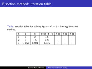
The document provides an overview of root-finding methods, including the bisection method, fixed-point method, and the Babylonian method for finding square roots. It discusses the iterative processes involved in these methods, their convergence rates, and includes exercises for better understanding. The bisection method is highlighted as fundamental despite its slower convergence, while fixed-point methods are analyzed for their conditions of existence and uniqueness.

1. Introduction to root finding
Sanjeev Kumar Verma
Department of Physics and Astrophysics
University of Delhi
Delhi, INDIA - 110007
sanjeevkumarverma.wordpress.com
Sanjeev Kumar Verma Introduction to root finding

2. Root finding
Introduction
Bisection method
Fixed point method
Newton’s method
Method of false position
Sanjeev Kumar Verma Introduction to root finding

3. Introduction
On a Babylonian clay tablet dated BC7289, a square is drawn
with its two diagonals and the diagonal to side ratio has been
written as 1.24, 51, 10.
Babylonians, unlike us, used sexagesimal number system. So,
the value is 1 + 24/60 + 51/602 + 10/603 = 1.41421296...
Exercise: What is the accuracy of this value?
Exercise: Can you calculate it without a calculator?
Exercise: Can you calculate it without using the standard
method based upon division and completion of square?
Sanjeev Kumar Verma Introduction to root finding

4. Babylonian method of finding square roots
As an example, let’s find
√
2.
Start with any guess. Say, the root is 1.
Babylonian method says that a better guess is average of the
old guess and the given number divided by the old guess.
So, new guess = average of 1 and 2/1 = 1.5.
Exercise. Take 1.5 as an old guess and calculate the new
guess.
Answer: average of 1.5 and 2/1.5 = 1.4167.
Repeating this process yields the series
{1, 1.5, 1.4166667, 1.4142157, 1.4142136, 1.4142136}
.
Sanjeev Kumar Verma Introduction to root finding

5. Babylonian method of finding square roots
Theorem: Let xn+1 = 1
2 xn + N
xn
. Then, xn → x for any x0
with sufficiently large n, where x =
√
N.
The idea is to start with a guess x0 and generate the series
{xn} = {x0, x1, x2, x3, x4, ...} using
xn+1 =
1
2
xn +
N
xn
. (1)
x0 is called initial guess. Each application of Eq. (1) is called
an iteration. xn is the value of the root after n iterations.
With successive iterations, the gap between xn+1 and xn goes
on becoming smaller and smaller. The difference between xn
and the true root x also goes on becoming smaller and smaller
with successive iterations. This is called convergence.
Sanjeev Kumar Verma Introduction to root finding

6. Exercises: Iterative methods
Ex. 1. Babylonian method of finding square roots illustrates
the key ideas of any iterative method. List them.
We have an initial solution.
We have an iterative formula.
Successive iterations give better approximations to the
solution.
An iterative method should converge towards the actual
solution.
Ex. 2. Try to develop a Babylonian like iterative method for
finding the cube root of a number. Use your intuition in
absence of any theoretical guidlines.
Sanjeev Kumar Verma Introduction to root finding

7. Bisection method: basic idea
The concept behind bisection method is illustrated with help
of following example.
Example Find the solution to the equation x2 = 2.
1 < 2 < 4
⇒ 1 <
√
2 < 2
So, the interval {1, 2} contains the root. Bisect the interval.
We get two new intervals: {1, 1.5} and {1.5, 2}. Which one
contains the root?
First interval, because 12 <
√
2
2
< 1.52 ⇒ 1 <
√
2 < 1.5.
Bisect the interval {1, 1.5} and repeat the procedure.
Each iteration will narrows down the root containing interval
by a factor of half successively. Make a nice table of iterations.
Ex. How do you select the root containing interval?
Hint: Function changes sign at the root.
Sanjeev Kumar Verma Introduction to root finding

8. Bisection method: iteration table
Table: Iteration table for solving f (x) = x2
− 2 = 0 using bisection
method.
n a b c=(a+b)/2 f(a) f(b) f(c)
1 1 2 1.5 - + +
2 1 1.5 1.25 - - +
3 1 .250 1.500 1.375 - + -
Sanjeev Kumar Verma Introduction to root finding

9. Bisection method: iteration table
Table: Iteration table for solving f (x) = x2
− 2 = 0 using bisection
method.
n a b c=(a+b)/2 f(a) f(b) f(c)
1 1 2 1.5 - + +
2 1 1.5 1.25 - - +
3 1 .250 1.500 1.375 - + -
4 1.3750 1.5000 1.4375 - + +
5 1.3750 1.4375 1.40625 - + -
6 1.40625 1.43750 1.42188 - + +
7 1.40625 1.42188 1.41407 - + -
8 1.41406 1.42188 1.41797 - + +
9 1.41406 1.41797 1.41602 - + +
10 1.41406 1.41602 1.41505 - + +
11 1.41406 1.41504 1.41456 - + +
12 1.41406 1.41455 1.41431 - + -
13 1.41406 1.41431 1.41418 - + +
14 1.41418 1.41431 1.41425 - + +
15 1.41418 1.41425 1.41422 - + +
16 1.41418 1.41422 1.41420 - + -
17 1.41420 1.41422 1.41421 - +
Sanjeev Kumar Verma Introduction to root finding

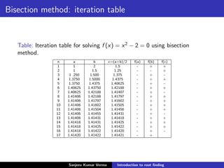
10. Bisection method: Estimate of convergence
Bisection method converge very slowly. How do we estimate the
number of iterations needed to solve an equation correct upto (say)
3, 4 or 5 places of decimal?
Suppose, we have to solve f (x) = 0 and the true solution is p. Let
[a, b] is the interval which contains the root.
Bisection method successively bisects the interval [a, b] into smaller
intervals [a1, b1], [a2, b2], [a3, b3] ... [an, bn] where
(bn − an) =
1
2n
(b − a). (2)
Bisection method successively approximates the root by
pn =
1
2
(an + bn) (3)
so that the sequence {pn} approaches p in the large n limit with
|pn − p| ≤
b − a
2n
. (4)
Actual error can be smaller than the above estimate.
Sanjeev Kumar Verma Introduction to root finding

11. Bisection method: Estimate of convergence
Eq. (4) is the required estimate of convergence.
Proof: Using Eq. (3), we have
pn − p =
1
2
(an + bn) − p
Since, |pn − p| < |pn − an|, we have
|pn − p| ≤
1
2
(an + bn) − an
=
1
2
(bn − an)
=
1
2n
(b − a)
Exercise What are the no. of iterations needed to determine
the root of equation x2 − 2 = 0 to an accuracy of 10−2 to
10−7?
accuracy 10−2 10−3 10−4 10−5 10−6 10−7
n 7 10 13 17 20 23
Sanjeev Kumar Verma Introduction to root finding

12. Bisection method: final comments
It is most fundamental method of root finding. When nothing
works, use it.
It comes with a guarantee of convergence.
Main drawback is the speed of convergence.
You can use it initially to narrow down the root containing
interval and then switch over to faster methods.
Ex. Solve x2 − 5 = 0, cos x − x = 0 and tan x = x using
bisection method to an accuracy of 10−3.
Sanjeev Kumar Verma Introduction to root finding

13. Fixed point method: basic idea
Consider following example:
x2
= 2
x2
− 1 = 1
(x − 1)(x + 1) = 1
x = 1 +
1
1 + x
(5)
x1 = 1 +
1
1 + x0
,
x2 = 1 +
1
1 + x1
,
x3 = 1 +
1
1 + x2
...
xn+1 = 1 +
1
1 + xn
. (6)
Sanjeev Kumar Verma Introduction to root finding

14. Fixed point method: basic idea
If x0 = 1, we have x1 = 1 + 1/2 = 1.5, x2 = 1 + 1/2.5 = 1.4
and so on. Essentially, we get the following sequence:
{xn} =
{1, 1.5, 1.4, 1.41667, 1.41379, 1.41429, 1.41420, 1.41422...}
7 iterations give you an accuracy of 10−5. Compare it with
bisection method.
Even if you start with x0 = 10, accuracy of 10−5 is achieved in
just 7 iterations!
Ex. Solve N = N0eλt + 3
λ for λ where N = 180, N0 = 100
and t = 1.
Hint: The iteration formula is λn+1 = 3/(180 − 100eλn ).
Solution: {λn} =
{1, −0.00326697, 0.0360515, 0.0393035, 0.0394782, 0.0394876,
0.0394881}.
Sanjeev Kumar Verma Introduction to root finding

15. Fixed point method: basic idea
The idea is to rewrite the equation f (x) = 0 as x = g(x). If
x = p is the root of f (x) = 0, it is called fixed point of g(x).
With this rearrangement, finding the root of f (x) is equivalent
to finding the fixed point of g(x).
Def. x = p is a fixed point of a function g(x) if g(p) = p.
Exercise: Find out the geometric meaning of the fixed point.
But, is there a guarantee that a fixed point always exists for a
function? If there is one, how to find the interval containing
it? How do you know that there will be only one fixed point in
the given root containing interval?
Ans. There is no guarantee for existence of a fixed point for a
function in the given interval! However, it’s existence is not
guided by your luck! There is a theorem for it.
Sanjeev Kumar Verma Introduction to root finding

16. Fixed point method: It fails here!
Let’s again try to solve x2 − 2 = 0.
Rewrite it as x2 + x − x − 2 = 0 and rearrange it to have
x = x2 + x − 2.
This gives you an iteration formula: xn+1 = x2
n + xn − 2.
Start with x0 = 1 and you get {xn} = {1, 0, −2, 0, −2, ...}. It
is not converging, it is oscillating!
Start with x0 = 2 and you get
{xn} = {2, 4, 18, 340, 115938...} : it is diverging!
What is wrong here? Can we diagnose the problem without
using mathematics?
If we can’t, let’s be mathematicians for a while!
Sanjeev Kumar Verma Introduction to root finding

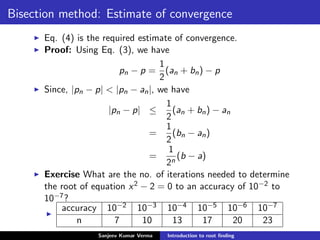
17. Fixed point theorem
(i) Consider a continuous function g(x) defined on the
interval [a, b]. If g(x) ∈ [a, b] ∀ x ∈ [a, b], ∃ a fixed point
p ∈ [a, b] defined as g(p) = p. (existence of fixed point)
(ii) If the function g(x) is differentiable and g (x) is bounded
from above in the interval [a, b] and |g (x)| ≤ k < 1 for some
positive number k, then the fixed point p is unique.
(condition for divergence or oscillation)
(iii)For any p0 ∈ [a, b], the sequence [pn] defined as
pn = g(pn−1)
converges to the unique fixed point p in [a, b]. (condition for
convergence)
Sanjeev Kumar Verma Introduction to root finding

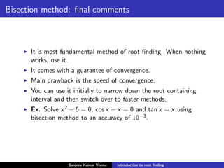
18. Fixed point theorem: application
Let g(x) = x2 + x − 2. Let x ∈ [0, 1]. Is g(x) ∈ [0, 1]? If yes,
there will be a fixed point in [0, 1].
Here, g(x) is a monotonically increasing function and
g(x) ∈ [−2, 0]. g(x) is completely outside the desired
interval! That was why you didn’t get the root in this case!
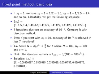
Now, take g(x) = 1 + 1
1+x . Let x ∈ [0, 1]. Is g(x) ∈ [0, 1]? If
yes, there will be a fixed point in [0, 1]. Otherwise, not.
Here, g(x) is monotonically decreasing function and
g(x) ∈ [1.5, 2]. So, there is no fixed point in [0, 1].
Is there a fixed point in [1, 2]?
If x ∈ [1, 2], then g(x) ∈ [1.33, 1.5] and hence g(x) ∈ [1, 2].
So, there will be a fixed point in [1, 2]!
Here, |g (x)| = 1
(1+x)2 < 1
4 which is always smaller than 1 in
[1, 2]. So, the fixed point is unique and there is guarantee of
convergence in this case.
Sanjeev Kumar Verma Introduction to root finding

19. Fixed point theorem: Proof
If you are not interested in proof of this theorem, I can give
you two motivations:
A corollary of the theorem will give you the order of
convergence of this method! So, you can calculate how many
iterations are needed to get the fixed point correct upto 5
places of decimals.
A question will definitely be asked based upon the fixed point
method in the finals!
Sanjeev Kumar Verma Introduction to root finding

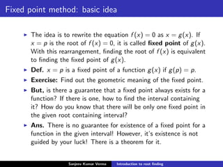
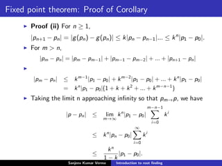
20. Fixed point theorem: Proof
(i) If a or b is a fixed point, then g(a) = a or g(b) = b.
If a and b are not fixed points, but there is a fixed point in
[a, b], then a < g(a) and g(b) < b. Why?
Let h(x) = g(x) − x. Then, h(a) = g(a) − a > 0 and
h(b) = g(b) − b < 0. Does this remind you of something?
Bisection method! ∃p ∈ (a, b) s.t.
h(p) = 0 ⇒ g(p) − p = 0 ⇒ g(p) = p. Hence, there exists a
fixed point p ∈ (a, b).
Sanjeev Kumar Verma Introduction to root finding

21. Fixed point theorem: Proof
(ii) Let g (x) ≤ k < 1. Let p and q are two fixed points in
(a, b). If p = q, then ∃ζ ∈ (p, q) s.t.
g(p) − g(q)
p − q
= g (ζ).
So,
|p − q| = |g(p) − g(q)| = |g (ζ)||p − q| ≤ k|p − q| < |p − q|
since k < 1. But, this is a contradiction! Hence, our
assumption is false: the fixed point is unique.
Sanjeev Kumar Verma Introduction to root finding

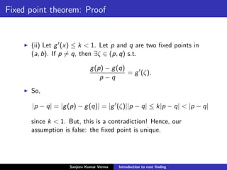
22. Fixed point theorem: Proof
(iii) Since g maps [a, b] into itself, the series pn = g(pn−1)
defined and pn ∈ [a, b] ∀ n.
Since, |g (x)| < k for all x, for each n we have
|pn −p| = |g(pn−1)−g(p)| = |g (ζn)||pn−1 −p| ≤ k|pn−1 −p|.
for some ζn ∈ (a, b).
So, |pn − p| ≤ k|pn−1 − p| ≤ k2|pn−2 − p| and so on.
Finally, |pn − p| ≤ kn|p0 − p|.
In the limiting case when n approaches infinity, kn → 0 and so
|pn − p| → 0 or pn → p.
Sanjeev Kumar Verma Introduction to root finding

23. Fixed point theorem: Corollary
(i) The error in pn is given by
|pn − p| ≤ kn max{p0 − a, b − p0}
(ii) Also, |pn − p| ≤ kn
1−k |p1 − p0| ∀ n ≥ 1.
Proof (i) Since, |pn − p| ≤ |p0 − p|, we have
|pn − p| ≤ kn
max{p0 − a, b − p0}
Why?
The p0 and p are between points a and b. So, the distance of
between p and p0 is always smaller than or equal to the
distance between p0 and a or b, whichever is maximum.
−−−−−−−−−−a−−−−−−−−−p0−−−−p−−−−−−−−−−−−b−−−−−−−−−−−
Sanjeev Kumar Verma Introduction to root finding

24. Fixed point theorem: Proof of Corollary
Proof (ii) For n ≥ 1,
|pn+1 − pn| = |g(pn) − g(pn)| ≤ k|pn − pn−1|... ≤ kn
|p1 − p0|.
For m > n,
|pm − pn| = |pm − pm−1| + |pm−1 − pm−2| + ... + |pn+1 − pn|
|pm − pn| ≤ km−1
|p1 − p0| + km−2
|p1 − p0| + ... + kn
|p1 − p0|
= kn
|p1 − p0|(1 + k + k2
+ ... + km−n−1
)
Taking the limit n approaching infinity so that pm→p, we have
|p − pn| ≤ lim
m→∞
kn
|p1 − p0|
m−n−1
i=0
ki
≤ kn
|pn − p0|
∞
i=0
ki
≤
kn
1 − k
|p1 − p0|.
Sanjeev Kumar Verma Introduction to root finding

25. Fixed point theorem: Application
Consider g(x) = 1 + 1
1+x . The fixed point of this function is
√
2.
|g (x)| = 1
(1+x)2 . For x ∈ [1, 2], we have |g (x)| < k = 1
4.
In six iterations, we have |p − pn| < 0.0002.
The speed of convergence, therefore, depends upon the
maximum value of |g (x)| viz. k.
In each iteration, the error in fixed point reduces by a factor
of k.
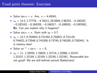
Ex. Can fixed point method converge at a slower rate than
bisection method?
Ans. For 0.5 < k < 1, fixed point method converges at a
slower rate than bisection method!
Lesson: Beware of simple minded thumb rules like bisection
method is slowest method. There is no way to escape
mathematical logic.
Sanjeev Kumar Verma Introduction to root finding

26. Fixed point theorem: Exercises
Solve tan x = x. Ans. x = 4.49341.
xn = {4.2, 1.77778, −4.76211, 20.0949, 2.96332, −0.180187,
−0.182163, −0.184205, −0.186317, −0.188503, −0.190768}.
Ex. Can you explain why it happens?
Solve cos x = x. Start with x0 = 0.7.
xn = {0.7, 0.764842, 0.721492, 0.750821, 0.731129,
0.744421, 0.73548, 0.741509, 0.73745, 0.740185, 0.738344}. It
is veeeery slow!
Solve xe−x + sin x − x = 0.
xn = {1., 1.20935, 1.29625, 1.31714, 1.32086, 1.32147,
1.32157, 1.32159, 1.32159, 1.32159, 1.32159}. Reasonable but
not good! We are still behind ancient Bablonians!
Sanjeev Kumar Verma Introduction to root finding

27. Newton’s method
The convergence speed the two methods we studied is much
slower as compared to the method used by Babylonians to
calculate square roots 10000 years ago!
Modern world was introduced to such a fast method only 300
years ago by Newton!
The iteration formula in newton’s method to calculate the
root of the function f (x) is
xn+1 = xn −
f (xn)
f (xn)
Ex. For f (x) = x2 − 2, we have
xn+1 = xn−
x2
n − 2
2xn
= xn−
xn
2
+
1
xn
=
xn
2
+
2
2xn
=
1
2
xn +
2
xn
.
This is the old Babylonian formula!
Sanjeev Kumar Verma Introduction to root finding

28. Newton’s method: Application
Let’s go back to the tedious example f (x) = cos x − x = 0
with x0 = 0.7.
The iteration formula is
xn+1 = xn −
cos xn − xn
(− sin xn − 1)
= xn +
cos xn − xn
1 + sin xn
.
The iterations give
{xn} = {0.7, 0.739436, 0.739085, 0.739085}: the root is
obtained to an accuracy of 10−6 in three iterations!
This is the fastest method we will study.
Sanjeev Kumar Verma Introduction to root finding

29. Newton’s Method: Applications
Now, you know that Newton’s method is behind the speed of
Babylonian method. So, derive Babylonian like formulas for
solving following problems:
Finding cube roots:
The iterative formula for x3 = N is
xn+1 =
1
3
2xn +
N
x2
n
.
Finding fixed point of a function g(x):
The fixed point of g(x) is the root of f (x) = g(x) − x.
Therefore, the iterative formula is
xn+1 = xn −
x − g(x)
1 − g (x)
.
Sanjeev Kumar Verma Introduction to root finding

30. Newton’s method: Logic behind it
Consider x = p is the root of f (x). So, f (p) = 0. Let,
f (p) = 0, xn be an approximation to the root and |xn − p| is
small.
Taylor expansion around x = xn:
f (x) = f (xn) + (x − xn)f (xn) +
(x − xn)2
2
f (xn) + ...
For x = p, we have
0 ≈ f (xn) + (p − xn)f (xn) +
(p − xn)2
2
f (xn) + ...
Since, |p − xn| is small and f (x) = 0, we have
p ≈ xn +
f (xn)
f (xn)
.
Hence, if xn is an approximation to root, a better approximation will
be
xn+1 = xn +
f (xn)
f (xn)
.
Sanjeev Kumar Verma Introduction to root finding

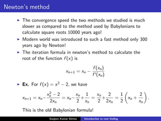
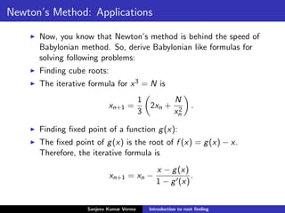
31. Newton’s method: A theorem
Consider a continuous and differentiable function f (x) defined
over an interval [a, b]. If p ∈ [a, b] is such that f (p) = 0 and
f (p) = 0, then there exists a δ > 0 such that Newton’s
method generates a sequence {xn} converging to p for any
initial guess x0 ∈ [p − δ, p + δ].
This theorem tell us about the inherent danger in Newton’s
method. If the value of δ is too small and the initial guess is
chosen outside the interval [p − δ, p + δ], the sequence {xn}
will diverge.
To sense this danger beforehand in practical applications, we
should know what δ is.
Sanjeev Kumar Verma Introduction to root finding

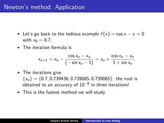
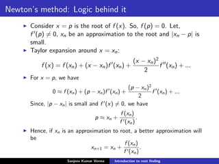
32. Newton’s method: Proof of the theorem
Newton’s method for finding the root of f (x) is equivalent to the
fixed point method for finding the fixed point of the function
g(x) = x − f (x)
f (x) .
Here,
g (x) = 1 −
f (x)f (x) − f (x)f (x)
[f (x)]2
=
f (x)f (x)
[f (x)]2
.
Since, f (p) = 0, g (p) = 0. So, |g (x)| vanishes at x = p. In the
interval [p − δ, p + δ] around p, |g (x)| will increase. We can always
choose a sufficiently small δ so that |g (x)| ≤ k < 1.
Let’s show that the interval [p − δ, p + δ] maps g(x) into itself. For
all x ∈ [p − δ, p + δ], |x − p| < δ.
So,
|g(x)−p| = |g(x)−g(p)| = |g (ζ)||(x −p)| ≤ k|x −p| < |x −p| < d
which implies that g(x) is also contained in the interval
[p − δ, p + δ] because g (x) exists and |g(x)| ≤ k < 1.
Hence, the series pn = g(pn−1) will converge to p according to fixed
point theorem.
Sanjeev Kumar Verma Introduction to root finding