The document discusses techniques for integrating trigonometric functions. It begins by reviewing definitions of trig functions like sine, cosine, tangent, and cotangent. It then provides examples of trig integrals using trig identities and u-substitution. Examples include integrals of sine, cosine, tangent, and secant functions. The document concludes by stating that practicing these types of integrals will help students perform well on exams involving calculus.
- The z-transform is a mathematical tool that converts discrete-time sequences into complex functions, analogous to how the Laplace transform handles continuous-time signals.
- Key properties and sequences that are transformed include the unit impulse δn, unit step un, and geometric sequences an.
- The z-transform is computed by taking the z-transform definition, which is an infinite summation, and obtaining closed-form expressions using properties like linearity and geometric series sums.
- Common transforms include U(z) for the unit step, 1/1-az^-1 for geometric sequences an, and expressions involving z, sinh/cosh, and sin/cos for exponential and trigonometric sequences.
The document discusses sampled functions and their z-transforms. It begins by explaining how sampling a continuous function at intervals of T produces a sequence of values. The z-transform of this sampled sequence is then related to the Laplace transform of the original continuous function. Specifically, the z-transform of the sampled sequence is equivalent to the Laplace transform with s replaced by z=esT. Examples are provided to illustrate this relationship between the pole locations of the two transforms.
The document discusses using z-transforms to solve difference equations. It provides examples of first and second order linear difference equations and explains how to solve them using z-transforms. The process involves taking the z-transform of each term in the difference equation, resulting in an algebraic equation that can be solved for the z-transform of the solution sequence. The inverse z-transform is then found to obtain the solution sequence. Partial fractions and residues can be used to invert z-transforms.
Welcome to International Journal of Engineering Research and Development (IJERD)IJERD Editor
The document summarizes research on coupled fixed point theorems in ordered metric spaces. It presents definitions of mixed monotone mappings and coupled fixed points. It then proves a new coupled fixed point theorem (Theorem 8) for mappings satisfying a contractive condition using the concept of g-monotone mappings. The theorem establishes the existence of a coupled fixed point when the mappings satisfy inequality (1). Finally, it presents coupled coincidence and common fixed point results (Theorems 9) for mappings satisfying integral type contractions.
The document summarizes research on accurate and total accurate dominating sets of interval graphs. It begins by introducing interval graphs and defining accurate and total accurate dominating sets. It then presents an algorithm to construct a minimum dominating set of an interval graph. Several theorems are provided about when the constructed dominating set is or is not an accurate dominating set or total accurate dominating set based on properties of the interval family and dominating set. The document focuses on characterizing accurate dominating sets of interval graphs.
These are slides of my lectures on numerical methods for graduate students. The lectures cover basic methods of finding roots of functions with one variable like bisection method, fixed point method, and Newton's method.
Using implicit differentiation we can treat relations which are not quite functions like they were functions. In particular, we can find the slopes of lines tangent to curves which are not graphs of functions.
This document discusses applying z-transforms to discrete systems to obtain the system's transfer function and output response. It begins by introducing z-transforms and their use in obtaining transfer functions for discrete systems. Transfer functions allow analyzing combinations of systems. The document provides examples of obtaining transfer functions for first and second order systems. It also covers obtaining the unit impulse and step responses from the transfer function. Finally, it discusses analyzing series combinations of systems by multiplying their individual transfer functions.
Fixed point theorem of discontinuity and weak compatibility in non complete n...Alexander Decker
The document presents a theorem about fixed points for six self-maps in a non-complete non-Archimedean Menger PM-space. The theorem proves that the six maps have a unique common fixed point under certain conditions, including:
1) The maps satisfy inequality conditions involving probabilistic metric functions.
2) One of the subspaces induced by two of the maps is complete.
3) The pairs of maps are R-weakly compatible.
The proof constructs a Cauchy sequence and uses properties of probabilistic metric spaces and weak compatibility to show the maps have a common fixed point.
11.fixed point theorem of discontinuity and weak compatibility in non complet...Alexander Decker
The document presents a theorem about fixed points for six self-maps in a non-complete non-Archimedean Menger PM-space. The theorem proves that the six maps have a unique common fixed point under certain conditions, including:
1) The maps satisfy inequality conditions involving probabilistic metric functions.
2) One of the subspaces induced by two of the maps is complete.
3) The pairs of maps are R-weakly compatible.
The proof constructs a Cauchy sequence and uses properties of probabilistic metric functions and the given conditions to show the sequence converges, establishing a common fixed point.
The document discusses the extension principle for generalizing crisp mathematical concepts to fuzzy sets. It defines the extension principle for mappings from cartesian products to universes. An example is provided to illustrate defining a fuzzy set in the output universe based on fuzzy sets in the input universes and the mapping between them. Fuzzy numbers are defined to have specific properties including being a normal fuzzy set, closed intervals for membership levels, and bounded support. Positive and negative fuzzy numbers are distinguished based on their membership functions. Binary operations are classified as increasing or decreasing, and it is noted the extension principle can be used to define the fuzzy result of applying increasing or decreasing operations to fuzzy inputs. Notation for fuzzy number algebraic operations is introduced. Several theore
The document provides an overview of neural networks and discusses:
- The background of neural networks including how they relate to brains and computational models.
- Abstractions of neurons and neural networks including McCullough-Pitts neurons and their representational completeness.
- Learnability in perceptrons including the perceptron training rule and convergence theorem for a perceptron to learn functions that are representable.
- An example of perceptron learning is shown for an "AND" function.
Moment closure inference for stochastic kinetic modelsColin Gillespie
This document discusses moment closure inference for stochastic kinetic models. It begins with an introduction to moment closure techniques using a simple birth-death process as a case study. It then discusses how to derive moment equations from the chemical master equation and how the deterministic model can be viewed as an approximation of the stochastic model by setting the variance to zero. The document also examines some limitations of moment closure approximations using examples of heat shock and p53-Mdm2 oscillation models. Finally, it presents a case study of using moment closure to model cotton aphid populations based on field data.
This document is a journey through pre-calculus functions told through photographs, math problems, and poetry. It discusses the challenges of learning difficult math concepts and emphasizes overcoming obstacles through perseverance. It uses examples like factoring polynomials and finding the domain of rational functions to illustrate key concepts. Poetry reflects on feeling overwhelmed but realizing the value of learning from mistakes to achieve success.
This document discusses various methods for solving first order differential equations, including:
1. Variable separable methods where the equation can be written as a function of x multiplied by a function of y.
2. Homogeneous equations where both sides are homogeneous functions of the same degree.
3. Exact equations where there exists an integrating factor.
4. Equations that can be transformed to an exact or separable form through substitution.
5. Linear equations that can be solved using an integrating factor that is a function of x.
This document discusses inverse functions, including exponential, logarithmic, and inverse trigonometric functions. It begins by defining an inverse function as two functions f and g where g(f(x)) = x and f(g(y)) = y. It then discusses how to find the inverse of a function by solving an equation like y = f(x) for x in terms of y. For a function to have an inverse, it must assign distinct outputs to distinct inputs. The document provides examples of finding inverses and discusses domains, ranges, and interpretations of inverse functions.
This document discusses regular perturbation theory through three chapters:
1. It defines key concepts like asymptotic sequences, asymptotic expansions, and order symbols used in perturbation theory.
2. It explains the fundamental ideas of regular and singular perturbations. Regular perturbations do not change the order of the problem when the perturbation parameter is set to zero, while singular perturbations do.
3. It provides examples of applying regular perturbation theory to solve algebraic equations. The technique involves expanding the solutions in powers of the perturbation parameter and solving the equations order-by-order. This allows approximating solutions even when exact solutions are not available.
This document provides a summary of key concepts in regular perturbation theory. It begins with an introduction and definitions related to regular and singular perturbations. Chapter 1 defines asymptotic sequences, asymptotic expansions, and order symbols like big-oh and little-oh notation. Chapter 2 discusses the fundamental ideas of perturbation like regularly and singularly perturbed problems. Chapter 3 solves sample regular perturbation problems like algebraic equations and differential equations to obtain asymptotic expansions of the solutions in terms of the perturbation parameter.
This document introduces the concept of order of an element modulo n and uses it to prove theorems about when an integer n satisfies n^2 + 1 or more generally satisfies a cyclotomic polynomial modulo a prime p. It begins by stating and proving the n^2 + 1 lemma, which says a prime p satisfies p | n^2 + 1 if and only if p ≡ 1 (mod 4). It introduces the concepts of order, primitive roots, and cyclotomic polynomials to generalize this result. It concludes by stating and proving a theorem about when a cyclotomic polynomial of an integer a is divisible by a prime p.
The document discusses Euler's generalization of Fermat's Little Theorem to composite moduli called the Theorem of Euler-Fermat. It explains that for any integer a coprime to a composite number m, a raised to the totient function of m (φ(m)) is congruent to 1 modulo m. It also provides formulas for calculating the totient function for prime powers and products of coprime integers. The Chinese Remainder Theorem, which states that a system of congruences with coprime moduli always has a solution, is introduced as well.
The document defines and discusses differential equations and their solutions. It begins by classifying differential equations as ordinary or partial based on whether they involve one or more independent variables. Ordinary differential equations are then classified as linear or nonlinear based on their form. The order and degree of a differential equation are also defined.
Solutions to differential equations can be either explicit functions that directly satisfy the equation or implicit relations that define functions satisfying the equation. Picard's theorem guarantees a unique solution through each point for first-order equations. The general solution to a first-order equation is a one-parameter family of curves, with a particular solution corresponding to a specific value of the parameter. An initial value problem specifies both a differential equation and
NONLINEAR DIFFERENCE EQUATIONS WITH SMALL PARAMETERS OF MULTIPLE SCALESTahia ZERIZER
In this article we study a general model of nonlinear difference equations including small parameters of multiple scales. For two kinds of perturbations, we describe algorithmic methods giving asymptotic solutions to boundary value problems.
The problem of existence and uniqueness of the solution is also addressed.
The document discusses linear partial differential equations (PDEs) with constant coefficients. It defines such PDEs and provides examples. It describes how to find the general solution of homogeneous linear PDEs with constant coefficients by finding the roots of the auxiliary equation. The general solution consists of the complementary function plus a particular integral. Methods for finding the particular integral when the right side consists of powers of x and y are also presented.
The document discusses solving systems of linear equations graphically. It provides examples of determining if an ordered pair is a solution by substituting into the equations and graphing the lines defined by the equations to find their point of intersection, which is the solution.
This document discusses ordinary differential equations (ODEs). It defines ODEs and differentiates them from partial differential equations. ODEs can be classified by type, order, and linearity. Initial value problems involve solving an ODE with initial conditions specified at a point, while boundary value problems involve conditions at boundary points. The document provides examples of solving first- and second-order initial value problems. It also discusses the existence and uniqueness of solutions to initial value problems under certain continuity conditions on the functions defining the ODE.
This document contains a math worksheet with 20 practice problems on integration using the substitution rule. It begins with an explanation of the substitution rule and its relationship to the chain rule. Students are asked to use substitutions to evaluate definite and indefinite integrals involving trigonometric, exponential, logarithmic and algebraic functions. The difficulty of the problems increases throughout the worksheet.
Integration by substitution allows difficult integrals to be evaluated by making a substitution of variables that simplifies the integrand. This technique involves changing both the variable of integration and the limits of integration. Key steps include identifying an appropriate substitution, determining the differential, and performing the integration with respect to the new variable before substituting back to the original. Extensive practice is important to master integration by substitution.
This document provides an overview of functions and function notation that will be used in Calculus. It defines a function as an equation where each input yields a single output. Examples demonstrate determining if equations are functions and evaluating functions using function notation. The key concepts of domain and range of a function are explained. The document concludes by finding the domains of various functions involving fractions, radicals, and inequalities.
Trigonometric substitutions can help evaluate integrals involving trigonometric functions. The document provides examples of using trigonometric substitutions to evaluate integrals of powers of sine and cosine functions. Specifically:
1) Integrals of powers of sine and cosine can be evaluated by rewriting the functions using trigonometric identities and then substituting variables. For example, sin5x can be rewritten as sinx(sin2x)2 and evaluated using the substitution u=cosx.
2) More complex integrals may require multiple steps and identities. For example, evaluating sin6x requires rewriting sin2x using an identity and then integrating four resulting terms.
3) Trigonometric substitutions allow rewriting integrals involving
The document discusses power series representations of functions. Power series allow functions that cannot be integrated, like ex2, to be approximated by polynomials which can be integrated. This allows integrals to be approximated to any degree of accuracy. Power series also allow irrational numbers like π to be expressed as an infinite decimal expansion. Power series approximations can be used to find approximate solutions to difficult differential equations.
This document discusses integration, which is the inverse operation of differentiation. It begins by explaining that integration finds the original function given its derivative, with the addition of a constant of integration. It then provides examples of basic integration techniques using a table of integrals. The document also outlines some rules for integrating sums and constant multiples of functions. Finally, it gives an example of using integration to solve an engineering problem involving the electric potential of a charged sphere.
This document discusses techniques for integrating trigonometric functions using u-substitution and trigonometric identities. It provides examples of integrating tan(x), cot(x), sec(x), csc(x) using the log rule with u-substitutions of u = ln(x), u = cos(x), and u = sec(x) + tan(x). It also evaluates integrals using Pythagorean identities and finds the average value of functions over an interval.
The document discusses finding a particular integral, which is any solution to an inhomogeneous differential equation. It describes trial solutions that can be used, including solutions with the same form as the right-hand side term. Examples are provided of finding particular integrals through substitution and equating coefficients. The general solution to an inhomogeneous equation is the sum of the particular integral and complementary function.
The document provides steps and examples for solving various types of word problems in algebra, including number, mixture, rate/time/distance, work, coin, and geometric problems. It also covers solving quadratic equations using methods like the square root property, completing the square, quadratic formula, factoring, and using the discriminant. Finally, it discusses linear inequalities, including properties related to addition, multiplication, division, and subtraction of inequalities.
This document discusses strategies for integration. It begins by noting that integration is more challenging than differentiation because it is not always obvious which integration technique to use. It then reviews commonly used techniques like substitution, integration by parts, and partial fractions. The document proposes a strategy for selecting techniques: 1) Simplify the integrand, 2) Look for obvious substitutions, 3) Classify the integrand form, 4) Try again using substitution or parts. It provides examples of applying these steps. The document also notes that not all integrals of continuous functions can be expressed in terms of elementary functions.
The document discusses the idea of integration by parts, which involves using the product rule in reverse to evaluate integrals that cannot be solved using other methods. It presents the integration by parts formula as u(x)v'(x)dx = u(x)v(x) - u'(x)v(x)dx and works through an example problem of evaluating the integral of xex dx using this formula. The example breaks the integral down into separate terms and shows that the overall integral equals xex - ex + C.
The document introduces slope fields as a way to visualize solutions to differential equations. It explains that a differential equation defines a family of curves rather than a single curve. The document then demonstrates how to use an online slope field calculator to plot the slope field for the differential equation dy/dx = 3x^2 and show that it corresponds to the family of curves y=x^3 + C, where C is any constant. It encourages exploring other differential equations using the slope field tool.
The document provides instructions for solving quadratic equations using two methods: factorizing and completing the square. It explains the steps to take to complete the square method, including halving the middle term to make a square, balancing the equation, isolating the square term on one side, and taking the square root. Students work through examples of solving quadratic equations with both methods and are given homework questions to practice.
This document provides an overview of topics covered in a differential equations course, including:
1. Review of integration by parts and partial fractions.
2. Discussion of integral curves and the existence and uniqueness theorem for differential equations.
3. Classification and methods for solving first and higher order linear differential equations, including separable, exact, integrating factors, Bernoulli, homogeneous with constant coefficients, and undetermined coefficients.
4. Brief introduction to additional solution methods like Euler's method, power series, and Laplace transforms.
5. Mention of solving systems of linear differential equations.
The document provides examples of solving literal equations by rearranging the equations to isolate the variable of interest. It explains that solving literal equations involves using inverse operations to get a letter alone on one side of the equation, rather than evaluating to a numerical solution. Additional examples demonstrate setting up and solving word problems involving literal equations, such as finding the constant in a direct variation relationship or using an equation to find the height of a wall.
The document provides examples of solving literal equations by rearranging the equations to isolate the variable of interest. It discusses solving equations to express variables like r, y, x, and H in terms of other variables. Additional examples show how to use literal equations to find constants in direct variation equations and to calculate heights using a bricklaying formula.
This document provides an overview of transformational geometry concepts for a test prep lesson, including definitions, examples, and practice problems. It reviews translations, reflections, rotations, and dilations by defining key terms, presenting rules and notation, and working through example problems. Students are instructed to complete a transformations packet in pairs during class and a test on these concepts will be given shortly. Reviewing notes and practice problems is recommended to prepare.
1) The document discusses integration as the reverse process of differentiation, and provides examples of integrating logarithmic and exponential functions.
2) Key points covered include integrating 1/x as ln(x), and exponential functions like e3x by using u-substitution and dividing the "tail" by the exponent.
3) The document also demonstrates integrating logarithmic expressions using u-substitution, letting the term in the denominator equal u and finding du.
This document contains a couple of problems from the textbook for Calc 1, Boise State, Fall 2014. It also explains the table method for evaluating complicated derivatives
Similar to Integrals with inverse trigonometric functions (20)
Three key points about three-dimensional geometry from the document:
1) Three-dimensional geometry developed in accordance with Einstein's field equations and is useful in fields like electromagnetism and for constructing 3D models using computer algorithms.
2) The document presents a vector-algebra approach to three-dimensional geometry, defining points as ordered triples of real numbers and discussing properties of lines and planes.
3) Key concepts discussed include the vector and Cartesian equations of lines and planes, direction cosines and ratios, angles between lines, perpendicularity, parallelism, and intersections. Formulas are provided for distances, divisions, and reflections.
A vector is a quantity with both magnitude and direction. There are two main operations on vectors: vector addition and scalar multiplication. Vector addition involves placing the tail of one vector at the head of another and drawing the third side of the resulting triangle or parallelogram. Scalar multiplication scales the length of a vector without changing its direction. Vectors can be represented using Cartesian components, where the magnitude and direction of a vector are given by its x, y, and z values relative to a set of perpendicular axes.
The document provides examples of non-verbal reasoning questions and their solutions. It includes number series, letter series, logical reasoning, and mathdoku puzzles. For the number series questions, the correct answer is choosing the option that continues the same pattern to fill in the missing term. The letter and logic series involve analyzing the relationship between letters or numbers to determine the missing element. The mathdoku puzzles require logically placing the numbers 1 to 5 in the grid so that each row and column uses each number, and the sums or products of the bold outlined groups equal the given hints.
The document provides several methods from Vedic mathematics for operations like squaring, multiplying, dividing, finding squares and square roots of numbers. Some key techniques discussed are:
1) A quick way to square numbers ending in 5 by splitting the answer into two parts and using the formula of multiplying the first number by one more than itself.
2) A method for multiplying where the first and last digits add to 10 by multiplying the first digit by the next number and combining with the product of the last digits.
3) Finding squares of numbers between 50-60 by adding the last digit to 25 and squaring the last digit.
4) Various sutras and techniques like vertically and crosswise,
The document discusses probability and experiments with random outcomes. It defines key probability concepts like sample space, events, and probability functions. It provides examples of common experiments with finite sample spaces like coin tosses, die rolls, and card draws. It also discusses experiments with infinite discrete sample spaces like repeated coin tosses until the first tail. The document establishes the basic properties and rules of probability, including that it is a function between 0 and 1, that probabilities of disjoint events add, and that probabilities of subsets are less than the original set.
The document defines matrices and provides examples of different types of matrices. It discusses key concepts such as rows, columns, dimensions, entries, addition, subtraction, and multiplication of matrices. It also covers special matrices like identity matrices, inverse matrices, transpose of matrices, and using matrices to solve systems of linear equations. The document is a comprehensive overview of matrices that defines fundamental terms and concepts.
This document discusses limits and continuity of functions. It introduces the concept of continuity and defines it using limits. Several examples of continuous and discontinuous functions are provided. Properties of continuous functions are discussed, including that the composition of continuous functions is continuous. Limits can be used to show a function is or is not continuous at a point. One-sided limits are also introduced and their relationship to continuity. The document concludes with a discussion of infinite limits.
1) The document defines and discusses the domains and ranges of inverse trigonometric functions such as sin-1x, cos-1x, and tan-1x.
2) The inverse functions are defined based on reflecting portions of the original trigonometric functions over the line y=x.
3) The domains and ranges of the inverse functions are restricted to ensure each inverse function is a single-valued function.
The document discusses several key concepts regarding derivatives:
(1) It explains how to use the derivative to determine if a function is increasing, decreasing, or neither on an interval using the signs of the derivative.
(2) It provides theorems and rules for finding local extrema (maxima and minima) of functions using the first and second derivative tests.
(3) It also discusses absolute extrema, monotonic functions, and the Rolle's Theorem and Mean Value Theorem which relate the derivative of a function to values of the function.
This document discusses different types of relations and functions. It defines equivalence relations, identity relations, empty relations, universal relations, one-to-one functions, onto functions, bijective functions, composition of functions, and invertible functions. It provides examples to illustrate these concepts.
The document defines matrices and their properties, including symmetric, skew-symmetric, and determinant. It provides examples of solving systems of equations using matrices and their inverses. It also discusses properties of determinants, including properties related to symmetric and skew-symmetric matrices. Inverse trigonometric functions are defined, including their domains, ranges, and relationships between inverse functions using addition and subtraction formulas. Sample problems are provided to solve systems of equations and evaluate determinants.
For the full video of this presentation, please visit: https://www.edge-ai-vision.com/2024/06/how-axelera-ai-uses-digital-compute-in-memory-to-deliver-fast-and-energy-efficient-computer-vision-a-presentation-from-axelera-ai/
Bram Verhoef, Head of Machine Learning at Axelera AI, presents the “How Axelera AI Uses Digital Compute-in-memory to Deliver Fast and Energy-efficient Computer Vision” tutorial at the May 2024 Embedded Vision Summit.
As artificial intelligence inference transitions from cloud environments to edge locations, computer vision applications achieve heightened responsiveness, reliability and privacy. This migration, however, introduces the challenge of operating within the stringent confines of resource constraints typical at the edge, including small form factors, low energy budgets and diminished memory and computational capacities. Axelera AI addresses these challenges through an innovative approach of performing digital computations within memory itself. This technique facilitates the realization of high-performance, energy-efficient and cost-effective computer vision capabilities at the thin and thick edge, extending the frontier of what is achievable with current technologies.
In this presentation, Verhoef unveils his company’s pioneering chip technology and demonstrates its capacity to deliver exceptional frames-per-second performance across a range of standard computer vision networks typical of applications in security, surveillance and the industrial sector. This shows that advanced computer vision can be accessible and efficient, even at the very edge of our technological ecosystem.
How to Interpret Trends in the Kalyan Rajdhani Mix Chart.pdfChart Kalyan
A Mix Chart displays historical data of numbers in a graphical or tabular form. The Kalyan Rajdhani Mix Chart specifically shows the results of a sequence of numbers over different periods.
Skybuffer SAM4U tool for SAP license adoptionTatiana Kojar
Manage and optimize your license adoption and consumption with SAM4U, an SAP free customer software asset management tool.
SAM4U, an SAP complimentary software asset management tool for customers, delivers a detailed and well-structured overview of license inventory and usage with a user-friendly interface. We offer a hosted, cost-effective, and performance-optimized SAM4U setup in the Skybuffer Cloud environment. You retain ownership of the system and data, while we manage the ABAP 7.58 infrastructure, ensuring fixed Total Cost of Ownership (TCO) and exceptional services through the SAP Fiori interface.
Northern Engraving | Nameplate Manufacturing Process - 2024Northern Engraving
Manufacturing custom quality metal nameplates and badges involves several standard operations. Processes include sheet prep, lithography, screening, coating, punch press and inspection. All decoration is completed in the flat sheet with adhesive and tooling operations following. The possibilities for creating unique durable nameplates are endless. How will you create your brand identity? We can help!
In the realm of cybersecurity, offensive security practices act as a critical shield. By simulating real-world attacks in a controlled environment, these techniques expose vulnerabilities before malicious actors can exploit them. This proactive approach allows manufacturers to identify and fix weaknesses, significantly enhancing system security.
This presentation delves into the development of a system designed to mimic Galileo's Open Service signal using software-defined radio (SDR) technology. We'll begin with a foundational overview of both Global Navigation Satellite Systems (GNSS) and the intricacies of digital signal processing.
The presentation culminates in a live demonstration. We'll showcase the manipulation of Galileo's Open Service pilot signal, simulating an attack on various software and hardware systems. This practical demonstration serves to highlight the potential consequences of unaddressed vulnerabilities, emphasizing the importance of offensive security practices in safeguarding critical infrastructure.
Ivanti’s Patch Tuesday breakdown goes beyond patching your applications and brings you the intelligence and guidance needed to prioritize where to focus your attention first. Catch early analysis on our Ivanti blog, then join industry expert Chris Goettl for the Patch Tuesday Webinar Event. There we’ll do a deep dive into each of the bulletins and give guidance on the risks associated with the newly-identified vulnerabilities.
Dandelion Hashtable: beyond billion requests per second on a commodity serverAntonios Katsarakis
This slide deck presents DLHT, a concurrent in-memory hashtable. Despite efforts to optimize hashtables, that go as far as sacrificing core functionality, state-of-the-art designs still incur multiple memory accesses per request and block request processing in three cases. First, most hashtables block while waiting for data to be retrieved from memory. Second, open-addressing designs, which represent the current state-of-the-art, either cannot free index slots on deletes or must block all requests to do so. Third, index resizes block every request until all objects are copied to the new index. Defying folklore wisdom, DLHT forgoes open-addressing and adopts a fully-featured and memory-aware closed-addressing design based on bounded cache-line-chaining. This design offers lock-free index operations and deletes that free slots instantly, (2) completes most requests with a single memory access, (3) utilizes software prefetching to hide memory latencies, and (4) employs a novel non-blocking and parallel resizing. In a commodity server and a memory-resident workload, DLHT surpasses 1.6B requests per second and provides 3.5x (12x) the throughput of the state-of-the-art closed-addressing (open-addressing) resizable hashtable on Gets (Deletes).
For the full video of this presentation, please visit: https://www.edge-ai-vision.com/2024/06/temporal-event-neural-networks-a-more-efficient-alternative-to-the-transformer-a-presentation-from-brainchip/
Chris Jones, Director of Product Management at BrainChip , presents the “Temporal Event Neural Networks: A More Efficient Alternative to the Transformer” tutorial at the May 2024 Embedded Vision Summit.
The expansion of AI services necessitates enhanced computational capabilities on edge devices. Temporal Event Neural Networks (TENNs), developed by BrainChip, represent a novel and highly efficient state-space network. TENNs demonstrate exceptional proficiency in handling multi-dimensional streaming data, facilitating advancements in object detection, action recognition, speech enhancement and language model/sequence generation. Through the utilization of polynomial-based continuous convolutions, TENNs streamline models, expedite training processes and significantly diminish memory requirements, achieving notable reductions of up to 50x in parameters and 5,000x in energy consumption compared to prevailing methodologies like transformers.
Integration with BrainChip’s Akida neuromorphic hardware IP further enhances TENNs’ capabilities, enabling the realization of highly capable, portable and passively cooled edge devices. This presentation delves into the technical innovations underlying TENNs, presents real-world benchmarks, and elucidates how this cutting-edge approach is positioned to revolutionize edge AI across diverse applications.
Main news related to the CCS TSI 2023 (2023/1695)Jakub Marek
An English 🇬🇧 translation of a presentation to the speech I gave about the main changes brought by CCS TSI 2023 at the biggest Czech conference on Communications and signalling systems on Railways, which was held in Clarion Hotel Olomouc from 7th to 9th November 2023 (konferenceszt.cz). Attended by around 500 participants and 200 on-line followers.
The original Czech 🇨🇿 version of the presentation can be found here: https://www.slideshare.net/slideshow/hlavni-novinky-souvisejici-s-ccs-tsi-2023-2023-1695/269688092 .
The videorecording (in Czech) from the presentation is available here: https://youtu.be/WzjJWm4IyPk?si=SImb06tuXGb30BEH .
What is an RPA CoE? Session 1 – CoE VisionDianaGray10
In the first session, we will review the organization's vision and how this has an impact on the COE Structure.
Topics covered:
• The role of a steering committee
• How do the organization’s priorities determine CoE Structure?
Speaker:
Chris Bolin, Senior Intelligent Automation Architect Anika Systems
Taking AI to the Next Level in Manufacturing.pdfssuserfac0301
Read Taking AI to the Next Level in Manufacturing to gain insights on AI adoption in the manufacturing industry, such as:
1. How quickly AI is being implemented in manufacturing.
2. Which barriers stand in the way of AI adoption.
3. How data quality and governance form the backbone of AI.
4. Organizational processes and structures that may inhibit effective AI adoption.
6. Ideas and approaches to help build your organization's AI strategy.
HCL Notes und Domino Lizenzkostenreduzierung in der Welt von DLAUpanagenda
Webinar Recording: https://www.panagenda.com/webinars/hcl-notes-und-domino-lizenzkostenreduzierung-in-der-welt-von-dlau/
DLAU und die Lizenzen nach dem CCB- und CCX-Modell sind für viele in der HCL-Community seit letztem Jahr ein heißes Thema. Als Notes- oder Domino-Kunde haben Sie vielleicht mit unerwartet hohen Benutzerzahlen und Lizenzgebühren zu kämpfen. Sie fragen sich vielleicht, wie diese neue Art der Lizenzierung funktioniert und welchen Nutzen sie Ihnen bringt. Vor allem wollen Sie sicherlich Ihr Budget einhalten und Kosten sparen, wo immer möglich. Das verstehen wir und wir möchten Ihnen dabei helfen!
Wir erklären Ihnen, wie Sie häufige Konfigurationsprobleme lösen können, die dazu führen können, dass mehr Benutzer gezählt werden als nötig, und wie Sie überflüssige oder ungenutzte Konten identifizieren und entfernen können, um Geld zu sparen. Es gibt auch einige Ansätze, die zu unnötigen Ausgaben führen können, z. B. wenn ein Personendokument anstelle eines Mail-Ins für geteilte Mailboxen verwendet wird. Wir zeigen Ihnen solche Fälle und deren Lösungen. Und natürlich erklären wir Ihnen das neue Lizenzmodell.
Nehmen Sie an diesem Webinar teil, bei dem HCL-Ambassador Marc Thomas und Gastredner Franz Walder Ihnen diese neue Welt näherbringen. Es vermittelt Ihnen die Tools und das Know-how, um den Überblick zu bewahren. Sie werden in der Lage sein, Ihre Kosten durch eine optimierte Domino-Konfiguration zu reduzieren und auch in Zukunft gering zu halten.
Diese Themen werden behandelt
- Reduzierung der Lizenzkosten durch Auffinden und Beheben von Fehlkonfigurationen und überflüssigen Konten
- Wie funktionieren CCB- und CCX-Lizenzen wirklich?
- Verstehen des DLAU-Tools und wie man es am besten nutzt
- Tipps für häufige Problembereiche, wie z. B. Team-Postfächer, Funktions-/Testbenutzer usw.
- Praxisbeispiele und Best Practices zum sofortigen Umsetzen
Essentials of Automations: Exploring Attributes & Automation ParametersSafe Software
Building automations in FME Flow can save time, money, and help businesses scale by eliminating data silos and providing data to stakeholders in real-time. One essential component to orchestrating complex automations is the use of attributes & automation parameters (both formerly known as “keys”). In fact, it’s unlikely you’ll ever build an Automation without using these components, but what exactly are they?
Attributes & automation parameters enable the automation author to pass data values from one automation component to the next. During this webinar, our FME Flow Specialists will cover leveraging the three types of these output attributes & parameters in FME Flow: Event, Custom, and Automation. As a bonus, they’ll also be making use of the Split-Merge Block functionality.
You’ll leave this webinar with a better understanding of how to maximize the potential of automations by making use of attributes & automation parameters, with the ultimate goal of setting your enterprise integration workflows up on autopilot.
Connector Corner: Seamlessly power UiPath Apps, GenAI with prebuilt connectorsDianaGray10
Join us to learn how UiPath Apps can directly and easily interact with prebuilt connectors via Integration Service--including Salesforce, ServiceNow, Open GenAI, and more.
The best part is you can achieve this without building a custom workflow! Say goodbye to the hassle of using separate automations to call APIs. By seamlessly integrating within App Studio, you can now easily streamline your workflow, while gaining direct access to our Connector Catalog of popular applications.
We’ll discuss and demo the benefits of UiPath Apps and connectors including:
Creating a compelling user experience for any software, without the limitations of APIs.
Accelerating the app creation process, saving time and effort
Enjoying high-performance CRUD (create, read, update, delete) operations, for
seamless data management.
Speakers:
Russell Alfeche, Technology Leader, RPA at qBotic and UiPath MVP
Charlie Greenberg, host
Connector Corner: Seamlessly power UiPath Apps, GenAI with prebuilt connectors
Integrals with inverse trigonometric functions
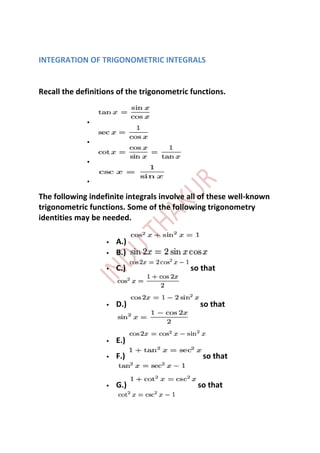
1. INTEGRATION OF TRIGONOMETRIC INTEGRALS
Recall the definitions of the trigonometric functions.
The following indefinite integrals involve all of these well-known
trigonometric functions. Some of the following trigonometry
identities may be needed.
A.)
B.)
C.) so that
D.) so that
E.)
F.) so that
G.) so that
2. It is assumed that you are familiar with the following rules of
differentiation.
These lead directly to the following indefinite integrals.
o 1.)
o 2.)
o 3.)
o 4.)
o 5.)
o 6.)
The next four indefinite integrals result from trig identities and u-
substitution.
o 7.)
3. o 8.)
o 9.)
o 10.)
We will assume knowledge of the following well-known, basic
indefinite integral formulas :
, where is a constant
. Integrals with Inverse Trigonometric Functions
1.
2.
11. These formulas, if effectively, practiced would help you perform
well in mathematics section especially calculus part of your
boards and entrances, thus helping you secure good marks in
your class XII exams and helping you secure a good rank in
entrance exams.
12. How to score well
Before you start the exam, utilize the first 15 minutes to scan
the paper. Read the question paper thoroughly before
jumping to write the answers.
Among the questions with internal choices, select the ones
that you plan to attempt, and frame skeletons of the answers
you are going to write for these questions.
Follow a pattern. For example, in case you start with long
answer questions, complete that section and only then move
to short or very short answer section.
Highlight the important points and write your answer in
points to enhance visibility.
Points to remember
Marks are deducted for
missing steps. So
remember to write down
all the steps.
Practice. Practice. Practice.
This is the mantra for
scoring good marks in CBSE
Class 12 Mathematics
Exam.
Make NCERT book your
bible. Revise and practise
all the problems solved in
the NCERT book.
13. Question: Integrate . Let
u = x-1
so that
du = (1) dx = dx .
In addition, we can "back substitute" with
x = u+1 .
Substitute into the original problem, replacing all forms of x,
getting
Question: Integrate . Let
u = 2x+3
so that
14. du = 2 dx ,
or
(1/2) du = dx .
In addition, we can "back substitute" with
x = (1/2)(u-3) .
Substitute into the original problem, replacing all forms of x,
getting
Question: Integrate . Let
u = x+2
15. so that
du = (1) dx = dx .
In addition, we can "back substitute" with
x = u-2 .
Substitute into the original problem, replacing all forms of x,
getting
Question: Integrate . Let
16. so that
.
In addition, we can "back substitute" with
.
Substitute into the original problem, replacing all forms of x,
getting
Question: Integrate . Use u-substitution. Let
u = 1+3e-x
so that (Don't forget to use the chain rule on e-x.)
17. du = 3e-x(-1) dx = -3e-x dx ,
or
(-1/3)du = e-x dx .
However, how can we replace the term e-3x in the original problem
? Note that
.
From the u-substitution
u = 1+3e-x ,
we can "back substitute" with
e-x = (1/3)(u-1) .
Substitute into the original problem, replacing all forms of x,
getting
(Recall that (AB)C = AC BC .)
18. Question: Integrate . Use u-substitution. Let
u = e2x+6ex+ 1
so that (Don't forget to use the chain rule on e2x.)
du = (2e2x+6ex) dx
= (2ex+x+6ex) dx
= (2exex+6ex) dx
= 2ex(ex+3) dx
19. = 2ex(3+ex) dx
or
(1/2) du = ex(3+ex) dx .
Substitute into the original problem, replacing all forms of x,
getting
(Do not make the following very common mistake :
. Why is this incorrect ?)
20. .
Question: Integrate . First, factor out e9x
from inside the parantheses. Then
(Recall that (AB)C = AC BC .)
(Recall that (AB)C = ABC .)
.
Now use u-substitution. Let
u = 27+e3x
so that (Don't forget to use the chain rule on e3x.)
du = 3e3x dx ,
21. or
(1/3) du = e3x dx .
Substitute into the original problem, replacing all forms of x , and
getting
.
Question: Integrate . Use u-substitution. Let
so that
22. ,
or
.
Substitute into the original problem, replacing all forms of ,
getting
.
Question: Integrate . First multiply by
, getting
.
.
.
Now use u-substitution. Let
so that
.
23. Substitute into the original problem, replacing all forms of ,
getting
.
Question: Integrate . Let
and
so that
and .
Therefore,
.
SOLUTION 6 : Integrate . Let
24. and
so that (Don't forget to use the chain rule when differentiating
.)
and .
Therefore,
.
Now use u-substitution. Let
so that
,
or
.
Then
25. +C
+C
+C.
Question: Integrate . Let
and
so that
and .
Therefore,
(Add in the numerator. This will replicate the
denominator and allow us to split the function into two parts.)
.
Question: Integrate . Let
and
so that
26. and .
Therefore,
.
Integrate by parts again. Let
and
so that
and .
Hence,
.
SOLUTION : Integrate . Use the power
substitution
so that
,
27. ,
and
.
Substitute into the original problem, replacing all forms of ,
getting
.
SOLUTION 6 : Integrate . Use the power
substitution
so that
,
,
and
.
Substitute into the original problem, replacing all forms of ,
getting
28. (Use polynomial division.)
.
Question: Integrate . Because the degree of the
numerator is not less than the degree of the denominator, we
must first do polynomial division. Then factor and decompose
into partial fractions, getting
(After getting a common denominator, adding fractions, and
equating numerators, it follows that ;
let ;
let .)
29. (Recall that .)
Question: Integrate . Because the degree of
the numerator is not less than the degree of the denominator,
we must first do polynomial division. Then factor and
decompose into partial fractions, getting
(After getting a common denominator, adding fractions, and
equating numerators, it follows that ;
let ;
let .)
30. .
SOLUTION : Integrate . Use the power substitution
so that
and
.
Substitute into the original problem, replacing all forms of ,
getting
(Use polynomial division.)
.
31. SOLUTION 4 : Integrate . Use the power
substitution
so that
,
,
and
.
Substitute into the original problem, replacing all forms of ,
getting
.
SOLUTION : Integrate . Use the power substitution
so that
32. and
.
Substitute into the original problem, replacing all forms of ,
getting
(Use polynomial division.)
.
Use the method of partial fractions. Factor and decompose into
partial fractions, getting
(After getting a common denominator, adding fractions, and
equating numerators, it follows that ;
let ;
let .)
(Recall that .)
.
33. Question: Integrate . Decompose into partial fractions,
getting
(After getting a common denominator, adding fractions, and
equating numerators, it follows that ;
let ;
let
;
it follows that and .)
.
Question: Integrate . Use u-substitution. Let
so that
.
34. Now rewrite this rational function using rules of exponents. Then
.
Substitute into the original problem, replacing all forms of ,
getting
.
Question: Integrate . First complete the square
in the denominator, getting
.
Now use u-substitution. Let
so that
.
In addition, we can "back substitute" with
35. .
Substitute into the original problem, replacing all forms of ,
getting
.
In the first integral use substitution. Let
so that
,
or
.
Substitute into the first integral, replacing all forms of , and use
formula 3 from the beginning of this section on the second
integral, getting
36. Integrate . First, use polynomial division to divide
by . The result is
.
In the second integral, use u-substitution. Let
so that
.
Substitute into the original problem, replacing all forms of ,
getting
(Now use formula 1 from the introduction to this section.)
.
SOLUTION : Integrate . Let
and
so that
and .
Therefore,
37. .
Use integration by parts again. let
and
so that
and .
Hence,
.
To both sides of this "equation" add , getting
.
Thus,
(Combine constant with since is an arbitrary
constant.)
.
Question: Integrate . Use integration by
parts. Let
and
so that
38. and .
Therefore,
.
Use integration by parts again. let
and
so that
and .
Hence,
.
From both sides of this "equation" subtract ,
getting
.
Thus,
(Combine constant with since is an arbitrary constant.)
39. INTEGRATION AS LIMIT OF A SUM AND ITS EVALUATION
Question: Use the limit definition of definite integral to evaluate
Divide the interval into equal parts each of length
for . Choose the sampling points to be the right-
hand endpoints of the subintervals and given by
for . The function is
.
Then the definite integral is
40. (Use summation rule 6 from the beginning of this section.)
(Use summation rules 5 and 1 from the beginning of this section.)
(Use summation rule 2 from the beginning of this section.)
.
Application of Integrals
41. Q. 1. Find the area of the region in the first quadrant
enclosed by the x-axis, the line y = x and the circle
Q. 2. Find the area of the region bounded by the ellipse
.
Q. 3. Find the area of the region bounded by the parabola
y = x2 and y = .
Q. 4. Find the area of the smaller part of the circle x2 + y2 =
a2 cut off by the linex= .
Q. 5. Using integration, find the area of the region bounded
by the triangle whose vertices are (1, 0), (2,2) and (3, 1).
Q. 6. Prove that the curves y2 = 4x and x2 = 4y divide the
area of the square bounded by x=0, x=4, y=4 and y=0 into
three equal parts.
Q. 7. Sketch the graph of y=
Q. 8. Using the method of integration, find the area
bounded by the curve .
Q. 9. Find the area of the smaller region bounded by the
ellipse .
Q. 10. Using integration, find the area of the triangular
region, the equations of whose sides are y=2x + 1, y=3x +1
and x = 4.
Q. 11. Find the area of the region
42. Q. 12. Find the area of the region between the circles x2 +
y2 = 4 and (x – 2)2 + y2 = 4.
Q. 13. Find the area bounded by the ellipse and
2 2 2
the co-ordinates x = ae and x = 0, where b =a (1 – e ) and
e<1.
Q. 14. Find the area bounded by the curve y2 = 4a2(x – 1)
and the lines x = 1and y = 4a.
Q. 15. Using integration, find the area of the region
bounded by the following curves, after making a rough
sketch: y = 1 +
Q. 16. Draw a rough sketch of the curves y = sinx and y =
cosx as x varies from o to and find the area of the
region enclosed by them and x-axis.
Q. 17. Find the area lying above x-axis and included
between the circle x2+ y2 = 8x and the parabola y2 = 4x.
Q. 18. Using integration find the area of the triangular
region whose sides have the equations y = 2x + 1, y = 3x +
1 and x = 4.
Q. 19. Find the area enclosed between the parabola y2 =
4ax and the line y = mx.
Q. 20. Find the area of the region bounded by the
parabolas y2 = 4 ax and x2 = 4 by
(NCERT)
Question 12: [ use: sin2x = 1- cos2x, ans. is x – sinx+c]
43. Question 14: [ Use: 1+sin2x= (cosx+sinx)2 , put
cosx+sinx = t , ans.is -1/(cosx+sinx)+c ]
Question 18: dx [use: cos2x = cos²x-sin²x , ans.tanx+c]
Question 22: [multiply & divide by sin(a-b), write
sin(a-b) = sin{(x-b)-(x-a)} in Nr., use formula of sin(A-B).ans. is
+c ]
Question 23: is equal to [(A) ]
A. tan x + cot x + C B. tan x + cosec x + C C. − tan x + cot x + C
D. tan x + sec x + C
Question 24: equals [(B) ]
A. − cot (exx) + C B. tan (xex) + C C. tan (ex) + C D. cot (ex) + C
Question 5: * Put x² = t , ans. is (3/2√2)tan-1(√2X²) +C +
Question 9: [Put tanx = t, ans. is log|tanx+ |+c]
Question 14: [ Dr. Can be written as =
= , ans. is sin-1( )+c ]
Question 17: [ + dx, put x²-1=t in 1st
integral, ans. is +2 log|x+ | +c ]
Question 18: [ let 5x-2 = P.d/dx(1+2x+3x²)+Q, P=5/6 &
Q=-11/3 , Ans. is 5/6 log (1+2x+3x²) – (11/3√2) tan-1( ) +c]
44. Question 25: equals *Dr. √–(4x²-9x)⇨ )² ,
(B)]
A B C D
Question 3: [ by partial fraction, A/(x-1)+B/(x-
2)+C/(x-3) ⇨A=1,B=-5 & C=4, ans. is log|x-1|-5log|x-2+4log|x-3|+c]
Question 8: [ A/(x-1)+B/(x-1)2 +C/(x+2)⇨ A=-C=2/9,
B=1/3, Ans. is 2/9log| |-1/3(x-1) +c]
Question 10: [same as Q.3, A=-1/10,B=5/2 & C=-24/5,
Ans. is 5/2 log|x+1|-1/10log|x-1|-12/5log|2x+3|+c ]
Question 12: [after division, we get x+ ⇨A=1/2,
B=3/2 , ans. is x²/2+1/2log|x+1|+3/2log|x-1|+c ]
Question 15: [ A/(x+1)+B/(x-1)+Cx+D/(x²+1)⇨ A=-
1/4,B=1/4,C=0 & D=-1/2 , ans. is ¼ log| |-1/2 tan-1x+c ]
Question 17: [Hint: Put sin x = t, ans.is log| |+c]
Question 18: [ put x²=y , , after dividing , we
get , 1- , by partial fraction A/(y+3) +B/(y+4) ⇨ A=-1, B=3,
ans. is x+(2/√3)tan-1(x/√3)-3tan-1(x/2) +c ]
Question 23: A. [(A) , multiply &
2
divide by x, put x = t, by partial fraction.]
45. B. C. D.
Question 5: x log 2x [integral by parts, (log2x).x²/2- ) dx
⇨ (log2x).x²/2 – x²/4+c ]
Question 14: [ integral by parts, (logx)².x²/2-
2
.1/x](x /2)dx , again by parts ⇨ (logx)².x²/2- [log x.(x²/2)-
] ⇨ (logx)².x²/2- x2/2(logx)+(1/4)x2 +c]
Question 6: [ ⇨ –
(9/2)log|(x+2)+ +c ]
Question 7: [ )2 ] ⇨(2x-3)/4
+(13/8)sin-1 (2x-3)/√3 +c +
Question 20: [ , by parts
⇨xex -ex – 4/п[cos(пx/4)] at x=0 to 1⇨ 1+4/п - 2√2/п ]
Question 4: [ ans. is 16/15(2+√2) +
Question 6: [ Dr. (17/4)- (x-1/2)² ⇨ (1/√17)log| |
Put x=0 to 2 ⇨ (1/√17) log( )]
Question 8: [by parts , ans is (e2/4)(e²-2) ]
Question 9:The value of the integral is A. 6 B. 0 C. 3 D. 4
-1
[ put x=sinѲ , limit will change from Ѳ=sin 1/3 when x=1/3 &
Ѳ=п/2 when x=1, ⇨ dѲ , put cotѲ=t, again
limit will change from √8 to 0 ans. is (A) =6]
46. IMPORTANT PROPERTIES OF DEFINITE INTEGRALS:
1. =
2. = a<c<b
3. =
4. =
5. = +
6. =2 , if f(2a-x) = f(x)
= 0 , if f(2a-x) = - f(x)
7. = 2 , if f is an even function i.e., f-x) = f(x)
= 0, if f is an odd function i.e., f(-x) = -f(x).
Question 6: [ ⇨ 9]
Question 10: [
=
⇨ -
=- ]
Question 12: [use property 4.⇨2I = . =2п ]
Question 15: [ use property 4. ⇨ 2I = =0 ]
Question 16: [ use property 4. ⇨ 2I =
⇨ I= =2 (BY PROP.6)= 2I1 …..(i) , where I1
= (by using prop. 4) ⇨ 2I1 =
⇨ - = I2 - п/2.log2 …..(ii) , where I2
= = (put 2x=y) = (by
prop. 6), from (i) & (ii) we get I = - п log2. ]
Question 19: Show that if f and g are defined
as and
47. [ by prop. 4 ⇨ I = = =
(according to given part) ⇨ I = 2 ]
Question 21:The value of is A. 2 B. C. 0 D.
[ use prop. 4 ⇨ 2I = =0 ]
Misc. Question 3: [Hint:Put ,ans. Is -2/a +c]
Question 4: [ put x= , ans. Is – ]
Question 5:
* ans. Is 2√x- 3x1/3 +6x1/6 -
6log|x1/6 +1| +c ]
Question 10: [ Nr. can be written as
2 2
(1-2sin xcos x)(-cos2x), ans. Is -1/2 sin2x +c ]
Question 11: [ same as Ques. 22]
Question 15: [ put cosx =y , ans. Is -1/4 cos4x +c ]
Question 16: [ put t = x4+1 , ans. Is ¼ log| x4+1| +c ]
Question 18: [ Dr. = sin4x cos + sin3xcosxsin =
sin4x(cos + cotxsin ) ( by using formula of sin(A+B)) , put t= cos
+ cotxsin , ans. Is -2/sin . +c ]
Question 19: [ use sin-1√x + cos-1√x =п/2 ⇨
48. 2/ dx – x , put √x= t, integrate by parts & use
formula of dt , ans. Is 4/п{ sin-1√x+ } –x +c]
Question 20: [ put x2 = cosy , use cos2y= (1+cos2y)/2, ans. Is
-2 √(1-x) + cos-1√x + √x . √(1-x) +c ]
Question 21: [use (f(x)+f’(x))dx , sin2x = 2sinx.cosx &
2 x
1+cos2x = 2cos x , ans. Is e tanx +c ]
Question 22: [ by partial fraction , we get A/(x+2) +
B/(x+1) +C/(x+1)2 ⇨ A=3, B=-2 & C=1, ans. Is log - (X+1)-1 +c ]
*Question 24: [ after simplification,we
integrate . log(1+ ) dx , put x = tanѲ , then put sinѲ=t (by
parts) , ans. Is -1/3 (1+ )3/2 { log(1+ )-2/3 } +c ]
Question 25: [ same as Ques. 21, ans. Is eп/2 ]
Question 26: [ divide Nr. & Dr. by cos4x , put tan2x =
y & limit will change from 0 to 1, ans. Is п/8 ]
Question 27: [ use sin2x = 1 – cos2x , Nr. Can be
written as 4-3cos2x-4 ⇨ -п/6+ 4/3 dx , put tanx = t,
limit will change from 0 to ∞, ans. Is п/6 or we can do it by another
method ( by partial fraction) divide Nr. & Dr. by cos2x , put tanx = t]
Question 28: [ put sinx-cosx=t ∵ sin2x=1-(sinx-cosx)2
Limit will change from –(√3-1)/2 to (√3-1)/2 ⇨ ∵ even
fn. , ans. Is 2 ]
49. Question 30: [ put sinx-cosx = t, same as Ques. 28 ,
limit will change from -1 to 0, ans. Is 1/40 log9 ]
Question 31: [ use sin2x formula , put sinx=t ,
integrate by parts , ans. Is п/2 -1 ]
Question 32: [ use prop. 4 ⇨ 2I = dx=
- , ans. Is ]
Question 33: [ +
+ dx+ dx + dx = 19/2 ]
Question 34: [ by partial fraction A/x +B/x2
+C/(x+1) ⇨ A= -1, B=1 & C=1 ]
Question 39: [ by parts ∫1. Sin-1xdx ]
Question 40: Evaluate dx as a limit of sum.
[nh =1, = +………+f((n-1)h)]
+………….. ]
. ( ∵ nh=1) =( ( =1 ]
Question 43:If then is equal to
A. B. C. D.
Question 44:The value of is A. 1 B. 0 C. – 1 D.
[Nr.=x+(x-1) & Dr.=1-x(1-x), use prop. 4 , it gives tan-1x+tan-1(x-1),B]
Definite Integral
Question 2: Find the area of the region bounded by y2 = 9x, x = 2, x
= 4 and the x-axis in the first quadrant.
50. Question 5:Find the area of the region bounded by the ellipse
Question 6:Find the area of the region in the first quadrant
enclosed by x-axis, line and the circle
Question 7:Find the area of the smaller part of the circle x2 + y2 = a2
cut off by the line
Question 9:Find the area of the region bounded by the parabola y =
x2 and
Question 10:Find the area bounded by the curve x2 = 4y and the line
x = 4y – 2
Question 1:Find the area of the circle 4x2 + 4y2 = 9 which is interior
to the parabola x2 = 4y
Question 2:Find the area bounded by curves (x – 1)2 + y2 = 1 and x2 +
y2 = 1
Question 5:Using integration find the area of the triangular region
whose sides have the equations y = 2x +1, y = 3x + 1 and x = 4.
Question 4:Using integration finds the area of the region bounded
by the triangle whose vertices are (–1, 0), (1, 3) and (3, 2).
Question 6:Smaller area enclosed by the circle x2 + y2 = 4 and the
line x + y = 2 is
A. 2 (π – 2) B. π – 2 C. 2π – 1 D. 2 (π + 2)
Question 7:Area lying between the curve y2 = 4x and y = 2x is
A. B. C. D.
Question 4:Sketch the graph of and evaluate
Question 8:Find the area of the smaller region bounded by the
ellipse and the line
Question 11:Using the method of integration find the area bounded
by the curve
51. [Hint: the required region is bounded by lines x + y = 1, x – y = 1, – x
+ y = 1 and – x – y = 11]
Question 12:Find the area bounded by curves
Question 14:Using the method of integration find the area of the
region bounded by lines: 2x + y = 4, 3x – 2y = 6 and x – 3y + 5 = 0
Question 15:Find the area of the region
Question 17:The area bounded by the curve , x-axis and the
ordinates x = –1 and x = 1 is given by [Hint: y = x if x > 0 and y = –x2
2
if x < 0]
A. 0 B. C. D.
Question 18:The area of the circle x2 + y2 = 16 exterior to the
parabola y2 = 6x is
A. B. C. D.
Question 19:The area bounded by the y-axis, y = cos x and y = sin x
when
Integration Problems
1. ∫(2x3 + 5x + 1)e2x dx [ans. e2x(x3 – 3/2x2 + 4x – 3/2) + C ]
2. ∫cos2 x tan2 x dx [ x/2− 1/4 sin 2x + C]
3. ∫e cos 2x
sin x cos x dx [ (−1/4) ecos 2x + C]
4. dx [ ln |2 + tan x| + C]
5. [ x2/2 − 3x + 8 ln |x + 3| + C]
6. dx [ 1/3(x2 + 4)3/2 − 4(x2 + 4)1/2 + C]
7. dx [ 2/3 ln |1 + 3√x| + C]
52. 8. dx [x +ln|x|+1/2ln|x2+4|−1/2arctan(x/2)+c]
9. [2/3 sin3x – cosx+c]
10. [ (2 - √2)/3 ]
**Question: Integrate . Let
.
In addition, we can "back substitute" with
,
or
x = (4-u)2 = u2-8u+16 .
Then
dx = (2u-8) du .
In addition, the range of x-values is
,
so that the range of u-values is
,
or
53. .
Substitute into the original problem, replacing all forms of x,
getting
.
INTEGRATION AS LIMIT OF A SUM AND ITS EVALUATION
54. Question: Divide the interval into equal parts each of
length
for . Choose the sampling points to be the right-
hand endpoints of the subintervals and given by
for . The function is
.
Then the definite integral is
(Use summation rule 6 from the beginning of this section.)
55. (Use summation rules 5 and 1 from the beginning of this section.)
(Use summation rule 2 from the beginning of this section.)
.
.
SOLUTION : Divide the interval into equal parts each of
length
56. for . Choose the sampling points to be the right-
hand endpoints of the subintervals and given by
for . The function is
.
Then the definite integral is
(Use summation rule 6 from the beginning of this section.)
(Use summation rules 5 and 1 from the beginning of this section.)
57. (Use summation rule 2 from the beginning of this section.)
.
Question: Divide the interval into equal parts each of length
for . Choose the sampling points to be the right-
hand endpoints of the subintervals and given by
for . The function is
.
59. (Use L'Hopital's rule since the limit is in the indeterminate form of
.)
.
**Question: Integrate . First, split the function into
two parts, getting
(Recall that .)
(Use formula 2 from the introduction to this section on integrating
exponential functions.)
61. .
**SOLUTION : Integrate . First, use polynomial
division to divide by . The result is
.
In the third integral, use u-substitution. Let
so that
,
or
.
62. For the second integral, use formula 2 from the introduction to
this section. In the third integral substitute into the original
problem, replacing all forms of , getting
(Now use formula 1 from the introduction to this section.)
**Question: Integrate . First rewrite this
rational function as
.
Now use u-substitution. Let
.
so that
,
or
.
In addition, we can "back substitute" with
.
63. Substitute into the original problem, replacing all forms of ,
getting
=
**Question: Integrate . Because the degree of the
numerator is not less than the degree of the denominator, we
must first do polynomial division. Then factor and decompose
into partial fractions (There is a repeated linear factor !), getting
(After getting a common denominator, adding fractions, and
equating numerators, it follows that
64. ;
let ;
let ;
let
;
let
;
it follows that and .)
**Question: Integrate . Factor and
decompose into partial fractions (There is a repeated linear factor
!), getting
65. (After getting a common denominator, adding fractions, and
equating numerators, it follows that
;
let ;
let ;
let ;
let
.)
.
66. **SOLUTION : Integrate . Factor and decompose
into partial fractions (There are two repeated linear factors !),
getting
(After getting a common denominator, adding fractions, and
equating numerators, it follows that
;
let ;
let ;
let
;
let
;
it follows that and .)
67. .
**Question: Integrate . Begin by rewriting the
denominator by adding , getting
(The factors in the denominator are irreducible quadratic factors
since they have no real roots.)
68. (After getting a common denominator, adding fractions, and
equating numerators, it follows that
;
let
;
it follows that and and ;
let
it follows that and and .)
.
Now use the method of substitution. In the first integral, let
so that
.
In the second integral, let
69. so that
.
In addition, we can ``back substitute", using
in the first integral and
in the second integral. Now substitute into the original problems,
replacing all forms of , getting
70. (Recall that .)
.
**Solution: Integrate. U se the power substitution
so that
and
.
71. Substitute into the original problem, replacing all forms of ,
getting
(Use polynomial division.)
.
**Question: Integrate . Because we want to
simultaneously eliminate a square root and a cube root, use the
power substitution
72. so that
,
,
,
and
.
Substitute into the original problem, replacing all forms of ,
getting
(Use polynomial division. PLEASE INSERT A FACTOR OF 6 WHICH
WAS ACCIDENTLY LEFT OUT.)
73. .
**SOLUTION : Integrate . Remove the ``outside"
square root first. Use the power substitution
so that
,
,
,
and (Use the chain rule.)
74. .
Substitute into the original problem, replacing all forms of ,
getting
.
**SOLUTION : Integrate . Remove the cube root
first. Use the power substitution
75. so that
,
,
,
and (Use the chain rule.)
.
Substitute into the original problem, replacing all forms of ,
getting
.
76. **Question: Integrate . Remove the
``outside" square root first. Use the power substitution
so that
,
and (Use the chain rule.)
,
or
.
Substitute into the original problem, replacing all forms of ,
getting
78. ,
and
.
Substitute into the original problem, replacing all forms of ,
getting
.
Use the method of partial fractions. Factor and decompose into
partial fractions, getting (There are repeated linear factors!)
(After getting a common denominator, adding fractions, and
equating numerators, it follows that
;
let ;
79. let ;
let
;
let
;
it follows that and .)
(Recall that .)
80. .
**SOLUTION : Integrate . Use the power
substitution
so that
and
.
Substitute into the original problem, replacing all forms of ,
getting
(Use polynomial division.)
81. .
Use the method of partial fractions. Factor and decompose into
partial fractions, getting
(After getting a common denominator, adding fractions, and
equating numerators, it follows that
;
let ;
let ;
let
;
it follows that and and .)
82. .
DEFINITE INTEGRAL
Theory:
To find the area between two intersecting curves that only
intersect at two points, we first find the ‘x’ coordinates of the two
intersection points: x = a and x = b. Definite integrals give us the
area under each curve from x = a to b, then we subtract the two
areas to obtain the area between the curves. In the diagram below,
the area between the two graphs is shaded:
83. Area under a Curve
The area between the graph of y = f(x) and the x-axis is given by the
definite integral below. This formula gives a positive result for a
graph above the x-axis, and a negative result for a graph below the
x-axis.
Note: If the graph of y = f(x) is partly above and partly below the x-
axis, the formula given below generates the net area. That is, the
area above the axis minus the area below the axis.
Formula:
84. Example Find the area between y = 7 – x2 and the x-
1: axis between the values x = –1 and x = 2.
Example Find the net area between y = sin x and the
2: x-axis between the values x = 0 and x = 2π.
Area between Curves
The area between curves is given by the formulas below.
Formula 1:
85. for a region bounded above and below by y =
f(x) and y = g(x), and on the left and right by x =
a and x = b.
Formula 2:
for a region bounded left and right by x = f(y)
and x = g(y), and above and below by y = c and y
= d.
Example 1:1 Find the area between y = x and y = x2 from x = 1
to x = 2.
Example 2:1 Find the area between x = y + 3 and x = y2 from y
= –1 to y = 1.
86. Area Under a Curve
Definite Integrals
So far when integrating, there has always been a constant term
left. For this reason, such integrals are known as indefinite
integrals. With definite integrals, we integrate a function between
2 points, and so we can find the precise value of the integral and
there is no need for any unknown constant terms [the constant
cancels out].
87. The Area Under a Curve
The area under a curve between two points can be found by doing
a definite integral between the two points.
To find the area under the curve y = f(x) between x = a and x = b,
integrate y = f(x) between the limits of a and b.
88. Areas under the x-axis will come out negative and areas above the
x-axis will be positive. This means that you have to be careful when
finding an area which is partly above and partly below the x-axis.
You may also be asked to find the area between the curve and the
y-axis. To do this, integrate with respect to y.
Example
Find the area bounded by the lines y = 0, y = 1 and y = x2.
89. EXAMPLE 4: Find the area between the curve f (x) = cos п x
on the interval [0, 2].
SOLUTION:
STEP 1: Graph the function.
(See figure 3)
STEP 2: Set up the integrals
and evaluate.
Notice that the area we
have to find is in three figure 3
pieces. The intervals [0, .5]
and [1.5, 2] are above the x-
axis, and the interval [.5,
1.5] is below. Therefore, we
will need to have three
integrals. Also notice that
symmetry cannot be used in
90. this problem.
EXAMPLE 5: Find the area between the curves f (x) = 4 - x 2
and g (x) = x 2 - 4.
SOLUTION:
STEP 1: Graph the functions.
(See figure 4)
The reason for graphing the
two equations is to be able
to determine which function
is on top and which one is
on the bottom. Sometimes, figure 4
you can also determine the
points of intersection. From
this graph, it is cleat that f
(x) is the upper function, g
(x) is the lower function, and
that the points of
intersection are x = -2 and x
= 2.
STEP 2: Determine the points of intersection.
If you did not determine the points of intersection from the graph,
solve for them algebraically or with your calculator. To find them
algebraically, set each equation equal to each other.
91. 4 - x 2 = x 2 – 4 ⇨ -2x 2 = -8 ⇨ x 2 = 4 ⇨ x = -2 or x = 2
STEP 3: Set up and evaluate the integral.
Recall from early in the notes, when we were finding the area
between the curve and the x-axis, we had to determine the upper
and the lower curve. Then the area was defined to be the following
integral.
So the definite integral would be the following.
Now, let us evaluate the integral.
If you look at the graph of the two functions carefully, you should
have noticed that we could have used some symmetry when
setting up the integral. The region is symmetric with respect to
both the x- and the y-axis. If we had used the y-axis symmetry, the
resulting integral would have had bounds of 0 and 2, and we would
have had to take 2 times the area to find the total area. Here is this
integral.
92. If we had used both symmetries, the resulting integral would still
have bounds of 0 and 2, but the upper function would have been f
(x) and the lower function would be y = 0 (the x-axis). To find the
total area, we would have to take this area times 4. Here is this
integral.
EXAMPLE 7: Find the area between the curves x = y 3 and x = y 2
that is contained in the first quadrant.
SOLUTION: STEP 1: Graph the functions. (See figure 6)
Since both equations are x in terms of y, we will integrate with
respect to y. When integrate with respect to x, we have to
determine the upper function and the lower function. Now that we
are integrating with respect to y, we must determine what function
is the farthest from the y-axis. The function that is the farthest
from the y-axis is x = y 2. So that will be our upper curve. The lower
curve will be the curve that is nearest to the y-axis. In this case, it is
the function x = y 3.
93. figure 6
STEP 2: Find the points of intersection.
Set the two equations equal to each other.
y 2 = y 3 ⇨ y 2 - y 3 = 0 ⇨ y 2 (1 - y) = 0 ⇨ y = 0 or y = 1
STEP 3: Set up and evaluate the integral.
using definite integrals to find the area between two curves
From the figure we can easily get that the area of the shaded
portion spqr = area tpqu - area tsru.
This is equivalent to the area enclosed between the curve y = f(x),
94. the x-axis and the ordinates x=a and x = b Minus the area
enclosed between the curve y = g(x), the x-axis and the ordinates
x = a and x = b. this is expressed mathematically as follows:
a
Therefore, the area between the two curves can be expressed as
a
Example - 3
Find the area bounded by the curves y = x2 and y = 2x.
Solution:
Step 1: To find the region we need to sketch the graph and find
where the two curves intersect.
To find where the curves intersect, we will set them equal to
each other and solve for x.
2x = x2
X2 - 2x = 0
X(x - 2) = 0
X = 0 or x - 2 = 0
X = 0 or x = 2
Plugging x = 0 into y = 2x gives us y = 2(0) = 0
Plugging x = 2 into y = 2x gives us y = 2(2) = 4
Therefore, the curves intersect at the points (0, 0) and (2, 4)
95. Step 2: as we can see in the figure, we are to find the area of the
shaded portion oabdo.
Area oabdo = area of oabco - area of odbco.
= the area enclosed between the straight line y = 2x, x-axis, x = 0
and
X = 2 Minus the area enclosed between the curve y = x2, x-axis, x
= 0 and x = 2.
Step 3: solve the definite integral.
square units
Example - 4:
Find the area bounded by the curves x2 = 4y and y2 = 4x.
Solution:
Step 1: Solve the given equations to find the points of
intersection.
(1) x2 = 4y, (2) y2 = 4x
Squaring both sides of (1) gives us x4 = 16y2
Substituting y2 = 4x into this equation gives us
x4 = 16(4x)
96. x4 = 64x
x4 - 64x = 0
x(x3 - 64) = 0
x = 0 or x3 = 64
x = 0 or x = 4
Plugging x = 0 into x2 = 4y gives us 0 = 4y implies that y = 0
Plugging x = 4 into x2 = 4y gives us 16 = 4y implies that y = 4
therefore, the points of intersection are (0, 0) and (4, 4)
Step 2: Sketch the graph.
Step 3: Solve both equations for y and write the formula for
finding the area of the shaded region.
Y2 = 4x Y = 2
since this is the equation of the top line, this will be the first part
of our equation.
X2 = 4y Y = x2
since this is the equation of the bottom line, this will be the
second part of our equation.
(recall the formula )
97. Therefore, the area of the shaded portion Sq. Units
Area Bounded by Two Curves: See Figure 12.3-8.
Example 1
Find the area of the region bounded by the graphs of f (x)=x3 and
g(x )=x. (See Figure 12.3-9.)
98. Step 1. Sketch the graphs of f (x ) and g (x ).
Step 2. Find the points of intersection.
Step 3. Set up integrals.
99. Note: You can use the symmetry of the graphs and let area
Analternate solution is to find the area using a calculator. Enter
and obtain .
Example 2
Find the area of the region bounded by the curve y =ex, the y-axis
and the line y =e2.
Step 1. Sketch a graph. See Figure 12.3-10.
Step 2. Find the point of intersection. Set e2 =ex x =2.
Step 3. Set up an integral:
Or using a calculator, enter and obtain (e2 +1).
100. Example 3
Using a calculator, find the area of the region bounded by y = sin x
and between 0≤ x ≤ π.
Step 1. Sketch a graph. See Figure 12.3-11.
Step 2. Find the points of intersection.
Using the [Intersection] function of the calculator, the
intersection points are x =0 and x =1.89549.
Step 3. Enter nInt(sin(x ) &8211; .5x, x, 0, 1.89549) and obtain
0.420798 ≈ 0.421.
(Note: You could also use the function on your calculator
and get the same result.)
Example 4
Find the area of the region bounded by the curve x y =1 and the
lines y = –5, x =e, and x =e3.
Step 1. Sketch a graph. See Figure 12.3-12.
101. Step 2. Set up an integral.
Step 3. Evaluate the integral.
102. ASSIGNMENT OF INTEGRATION
Question 1 Evaluate: (i)** Integrate .[ Use the power
substitution
Put ]
** (iii) Integrate . [ Use the power substitution
Put ]
(iii) [answer is (2 - √2)/3 ]
(iv) ∫ dx[multiply÷ by sin(a-b)](v) dx
[multiply & divide by ] (Vi)∫ dx [by partial fraction]
(v) dx [ use ∫ex(f(x)+f’(x))dx+ (vi) dx [put sinx=
, cosx = , then put t=tanx/2. Answer is – ]
(vii) dx [ + = ∫+ve dx+∫ -ve dx ,
answer is 5/2п- 1/п2] (viii) [ write sin2x = 1-cos2x answer is
п/6] (ix) + dx * answer is √2 ] (x) dx [ put
x=atan2Ѳ , answer is a/2(п-2) ] (xi) dx [ use property dx
= dx , dx = dx ∵f(2a-x) = f(x) , then put t=tanx,
answer is п²/2√2 ] (xii) dx , where f(x) =|x|+|x+2|+|x+5|.
[ dx + dx , answer is 31.5 ] (xiii) Evaluate dx
[use (f(x)+f’(x))dx Question 2 Using integration, find the area of the
regions: (i) { (x,y): |x-1| ≤y ≤ }
103. (ii) *(x,y):0≤y≤x2+3; 0≤y≤2x+3; 0≤x≤3+
[(i) A= dx- dx - dx = 5/2 [
+ ] – ½ ] [(ii) dx + dx , answer is 50/3]
(iii) Find the area bounded by the curve x 2 = 4y & the line x = 4y – 2.
[A = dx - dx = 9/8 sq. Unit.]
**(iv) Sketch the graph of f(x) = ,evaluate dx
[hint: dx = dx + dx = 62/3.]
**Question 3 evaluate dx [ mult. & divide by , put 1+x
=A.(d/dx)(x2+x)+B ,find A=B=1/2, integrate]
104. Definite integral as the limit of a sum , use formula : dx
, where nh=b-a & n→∞ Question 4 Evaluate
) dx (ii) dx
[ use = 1 for part (i) , use formulas of special sequences, answer
is 6]
Some special case :
(1) Evaluate: [ put x+1=t²] (2) [ put x+1 = t² ]
(3) Evaluate: (4) Evaluate: [ put x=1/t for both]
(5) Evaluate: [ divide Nr. & Dr. By x2 , then write x²+1/x²=(x-1/x)²
+2 according to Nr. , let x-1/x=t]
(6) Evaluate dx [ let x=A(d/dx) ( 1+x-x²) +B]
(7) Integrating by parts evaluate =
(8) Evaluate dx = dx [ put
sinx=Ad/dx(sinx+cosx)+B(sinx+cosx)+C
If Nr. Is constant term then use formulas of sinx,cosx as Ques. No. 1 (vi) part]