The document presents a detailed examination of moment closure based parameter inference related to stochastic kinetic models, including methodologies for handling birth-death processes and dimerization models. It addresses the relationship between deterministic and stochastic representations, illustrating how moment equations are derived and utilized for parameter inference in various biological models. Case studies such as the heat shock model and the p53-mdm2 oscillation model highlight the complexities and challenges in applying moment closure approximations in different scenarios.

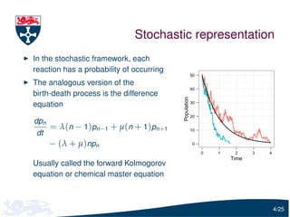
![Birth-death process
Birth-death model
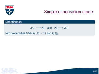
X −→ 2X and 2X −→ X
which has the propensity functions λX and µX .
Deterministic representation
The deterministic model is
dX (t )
= ( λ − µ )X (t ) ,
dt
which can be solved to give X (t ) = X (0) exp[(λ − µ)t ].
3/25](https://image.slidesharecdn.com/gillespie-120810171920-phpapp01/85/Moment-Closure-Based-Parameter-Inference-of-Stochastic-Kinetic-Models-3-320.jpg)
![Birth-death process
Birth-death model
X −→ 2X and 2X −→ X
which has the propensity functions λX and µX .
Deterministic representation
The deterministic model is
dX (t )
= ( λ − µ )X (t ) ,
dt
which can be solved to give X (t ) = X (0) exp[(λ − µ)t ].
3/25](https://image.slidesharecdn.com/gillespie-120810171920-phpapp01/85/Moment-Closure-Based-Parameter-Inference-of-Stochastic-Kinetic-Models-4-320.jpg)
![Moment equations
Multiply the CME by enθ and sum over n, to obtain
∂M ∂M
= [λ(eθ − 1) + µ(e−θ − 1)]
∂t ∂θ
where
∞
M (θ; t ) = ∑ e n θ pn ( t )
n =0
If we differentiate this p.d.e. w.r.t θ and set θ = 0, we get
dE[N (t )]
= (λ − µ)E[N (t )]
dt
where E[N (t )] is the mean
5/25](https://image.slidesharecdn.com/gillespie-120810171920-phpapp01/85/Moment-Closure-Based-Parameter-Inference-of-Stochastic-Kinetic-Models-6-320.jpg)
![The mean equation
dE[N (t )]
= (λ − µ)E[N (t )]
dt
This ODE is solvable - the associated forward Kolmogorov equation is
also solvable
The equation for the mean and deterministic ODE are identical
When the rate laws are linear, the stochastic mean and deterministic
solution always correspond
6/25](https://image.slidesharecdn.com/gillespie-120810171920-phpapp01/85/Moment-Closure-Based-Parameter-Inference-of-Stochastic-Kinetic-Models-7-320.jpg)
![The variance equation
If we differentiate the p.d.e. w.r.t θ twice and set θ = 0, we get:
dE[N (t )2 ]
= (λ − µ)E[N (t )] + 2(λ − µ)E[N (t )2 ]
dt
and hence the variance Var[N (t )] = E[N (t )2 ] − E[N (t )]2 .
Differentiating three times gives an expression for the skewness, etc
7/25](https://image.slidesharecdn.com/gillespie-120810171920-phpapp01/85/Moment-Closure-Based-Parameter-Inference-of-Stochastic-Kinetic-Models-8-320.jpg)
![Dimerisation moment equations
We formulate the dimer model in terms of moment equations
dE[X1 ] 2
= 0.5k1 (E[X1 ] − E[X1 ]) − k2 E[X1 ]
dt
2
dE[X1 ] 2 2
= k1 (E[X1 X2 ] − E[X1 X2 ]) + 0.5k1 (E[X1 ] − E[X1 ])
dt
2
+ k2 (E[X1 ] − 2E[X1 ])
where E[X1 ] is the mean of X1 and E[X1 ] − E[X1 ]2 is the variance
2
The i th moment equation depends on the (i + 1)th equation
9/25](https://image.slidesharecdn.com/gillespie-120810171920-phpapp01/85/Moment-Closure-Based-Parameter-Inference-of-Stochastic-Kinetic-Models-10-320.jpg)
![Deterministic approximates stochastic
Rewriting
dE[X1 ] 2
= 0.5k1 (E[X1 ] − E[X1 ]) − k2 E[X1 ]
dt
in terms of its variance, i.e. E[X1 ] = Var[X1 ] + E[X1 ]2 , we get
2
dE[X1 ]
= 0.5k1 E [X1 ](E[X1 ] − 1) + 0.5k1 Var[X1 ] − k2 E[X1 ] (1)
dt
Setting Var[X1 ] = 0 in (1), recovers the deterministic equation
So we can consider the deterministic model as an approximation to
the stochastic
When we have polynomial rate laws, setting the variance to zero
results in the deterministic equation
10/25](https://image.slidesharecdn.com/gillespie-120810171920-phpapp01/85/Moment-Closure-Based-Parameter-Inference-of-Stochastic-Kinetic-Models-11-320.jpg)
![Deterministic approximates stochastic
Rewriting
dE[X1 ] 2
= 0.5k1 (E[X1 ] − E[X1 ]) − k2 E[X1 ]
dt
in terms of its variance, i.e. E[X1 ] = Var[X1 ] + E[X1 ]2 , we get
2
dE[X1 ]
= 0.5k1 E [X1 ](E[X1 ] − 1) + 0.5k1 Var[X1 ] − k2 E[X1 ] (1)
dt
Setting Var[X1 ] = 0 in (1), recovers the deterministic equation
So we can consider the deterministic model as an approximation to
the stochastic
When we have polynomial rate laws, setting the variance to zero
results in the deterministic equation
10/25](https://image.slidesharecdn.com/gillespie-120810171920-phpapp01/85/Moment-Closure-Based-Parameter-Inference-of-Stochastic-Kinetic-Models-12-320.jpg)
![Simple dimerisation model
To close the equations, we assume an underlying distribution
The easiest option is to assume an underlying Normal distribution, i.e.
E[X1 ] = 3E[X1 ]E[X1 ] − 2E[X1 ]3
3 2
But we could also use, the Poisson
3
E[X1 ] = E[X1 ] + 3E[X1 ]2 + E[X1 ]3
or the Log normal
2 3
3 E [ X1 ]
E [ X1 ] =
E [ X1 ]
11/25](https://image.slidesharecdn.com/gillespie-120810171920-phpapp01/85/Moment-Closure-Based-Parameter-Inference-of-Stochastic-Kinetic-Models-13-320.jpg)
![Simple dimerisation model
To close the equations, we assume an underlying distribution
The easiest option is to assume an underlying Normal distribution, i.e.
E[X1 ] = 3E[X1 ]E[X1 ] − 2E[X1 ]3
3 2
But we could also use, the Poisson
3
E[X1 ] = E[X1 ] + 3E[X1 ]2 + E[X1 ]3
or the Log normal
2 3
3 E [ X1 ]
E [ X1 ] =
E [ X1 ]
11/25](https://image.slidesharecdn.com/gillespie-120810171920-phpapp01/85/Moment-Closure-Based-Parameter-Inference-of-Stochastic-Kinetic-Models-14-320.jpg)

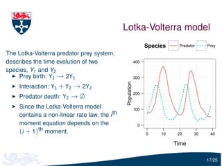
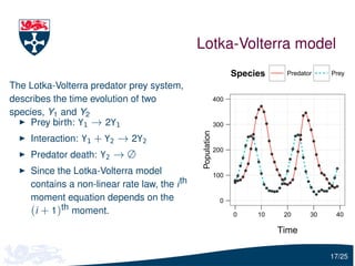
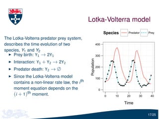
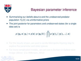
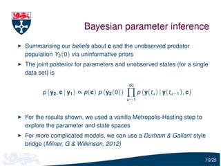
![Parameter estimation
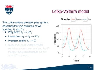
Let Y(tu ) = (Y1 (tu ), Y2 (tu )) be the vector of the observed predator
and prey
To infer c1 , c2 and c3 , we need to estimate
Pr[Y(tu )| Y(tu −1 ), c]
i.e. the solution of the forward Kolmogorov equation
We will use moment closure to estimate this distribution:
Y(tu ) | Y(tu −1 ), c ∼ N (ψu −1 , Σu −1 )
where ψu −1 and Σu −1 are calculated using the moment closure
approximation
18/25](https://image.slidesharecdn.com/gillespie-120810171920-phpapp01/85/Moment-Closure-Based-Parameter-Inference-of-Stochastic-Kinetic-Models-28-320.jpg)
![Parameter estimation
Let Y(tu ) = (Y1 (tu ), Y2 (tu )) be the vector of the observed predator
and prey
To infer c1 , c2 and c3 , we need to estimate
Pr[Y(tu )| Y(tu −1 ), c]
i.e. the solution of the forward Kolmogorov equation
We will use moment closure to estimate this distribution:
Y(tu ) | Y(tu −1 ), c ∼ N (ψu −1 , Σu −1 )
where ψu −1 and Σu −1 are calculated using the moment closure
approximation
18/25](https://image.slidesharecdn.com/gillespie-120810171920-phpapp01/85/Moment-Closure-Based-Parameter-Inference-of-Stochastic-Kinetic-Models-29-320.jpg)


![A. Basic Calculus [15]A1. The function f (x) is de…ned as.docx](https://cdn.slidesharecdn.com/ss_thumbnails/a-221114170355-6cba0b2a-thumbnail.jpg?width=640&height=640&fit=bounds)


