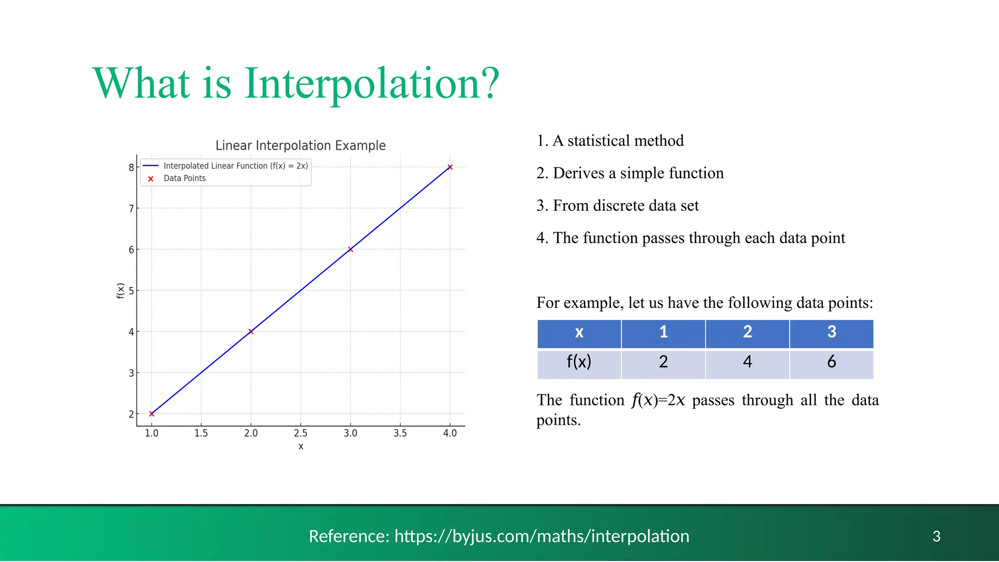
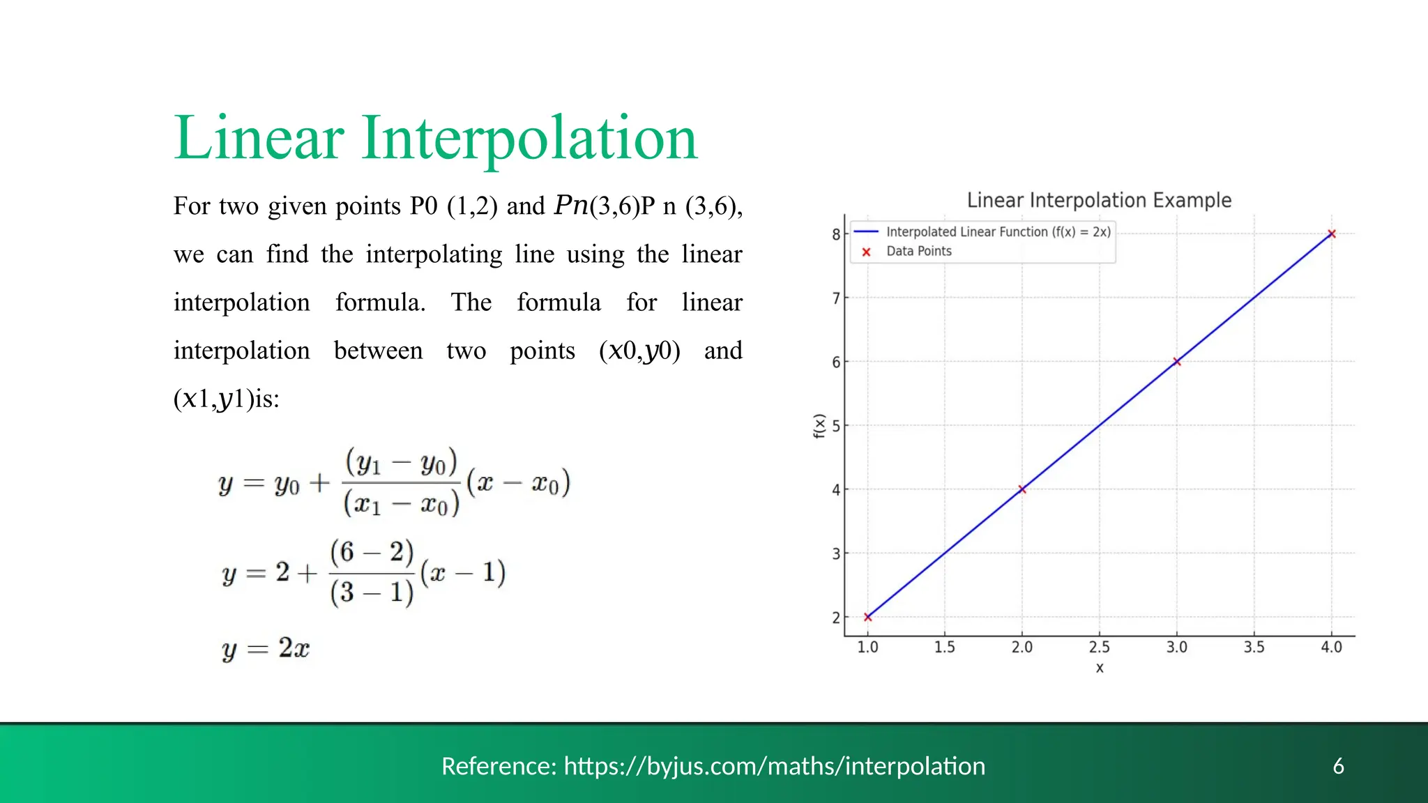
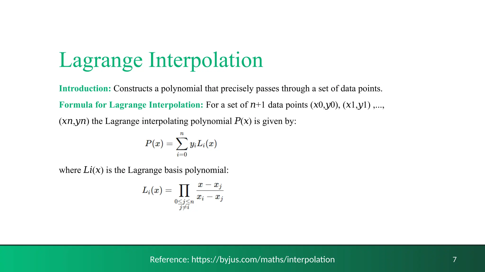
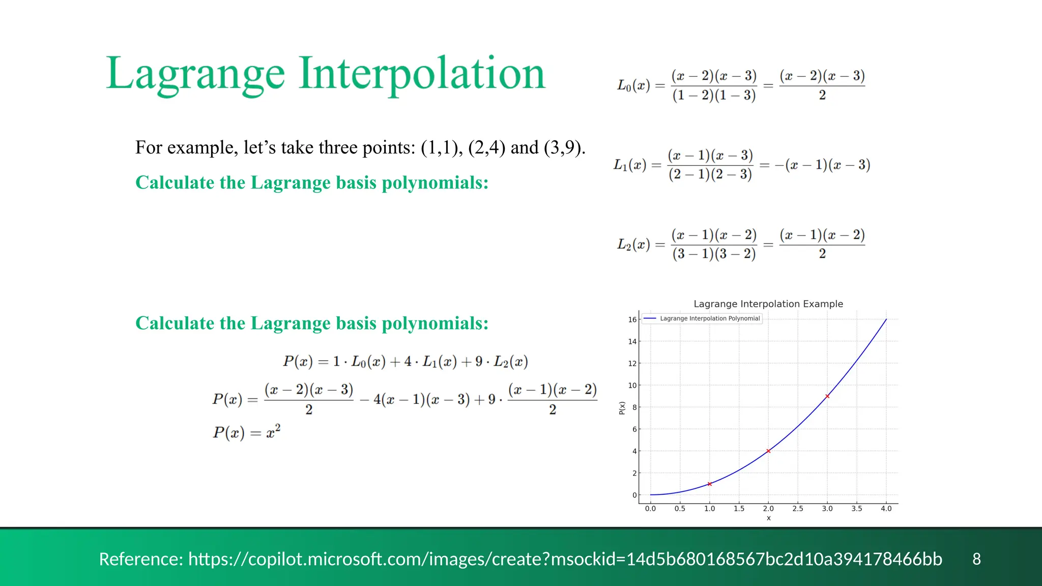
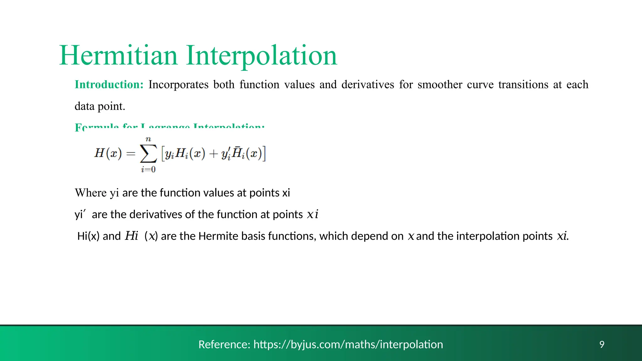
The document discusses various interpolation methods utilized in mathematics and computer graphics, including linear, polynomial, Lagrange, Hermitian, and spline interpolation. It details how these methods derive functions from discrete data points to create smooth transitions in graphics applications such as image scaling, rotation, and morphing. Overall, the document covers the advantages and limitations of interpolation techniques while providing examples and formulas for each type.

1. Interpolation Methods
Presented to:
Dr. Habiba Sultana
Assistant Professor
Presented By:
Md. Ashikur Rahman Ashik
Roll: 19102042
Reg. No: 7761
Department of Computer Science and Engineering
Jatiya Kabi Kazi Nazrul Islam University
Trishal, Mymensingh.

2. Contents
1. What is Interpolation?
2. Interpolation in Computer Graphics
3. Types of Interpolation
4. Linear Interpolation
5. Lagrange Interpolation
6. Hermitian interpolation
7. Spline Interpolation
8. Conclusion
9. References
2

3. What is Interpolation?
3
1. A statistical method
2. Derives a simple function
3. From discrete data set
4. The function passes through each data point
For example, let us have the following data points:
The function ( )=2 passes through all the data
𝑓 𝑥 𝑥
points.
x 1 2 3
f(x) 2 4 6
Reference: https://byjus.com/maths/interpolation

4. Interpolation in Computer Graphics
1. Image Scaling and Resizing
2. Image Rotation and Transformation
3. Color Interpolation in Shading
4. Morphing Effects
5. Animation and Motion Interpolation
4

5. Types of Interpolation
5
1. Linear Interpolation: Connects two known points with a straight line.
2. Polynomial Interpolation: Fits a polynomial through multiple data points.
3. Lagrange Interpolation: Constructs a polynomial that precisely passes through a set of data points.
4. Hermitian Interpolation: Incorporates both function values and derivatives for smoother curve
transitions at each data point.
5. Spline Interpolation: Uses piecewise polynomials to create a smooth curve between data points.

6. Linear Interpolation
For two given points P0​(1,2) and (3,6)P n​(3,6),
𝑃𝑛
we can find the interpolating line using the linear
interpolation formula. The formula for linear
interpolation between two points ( 0, 0) and
𝑥 𝑦
( 1, 1)is:
𝑥 𝑦
6
Reference: https://byjus.com/maths/interpolation

7. Lagrange Interpolation
Introduction: Constructs a polynomial that precisely passes through a set of data points.
Formula for Lagrange Interpolation: For a set of +1 data points ( 0, 0), ( 1, 1) ,...,
𝑛 𝑥 𝑦 𝑥 𝑦
( , ) the Lagrange interpolating polynomial ( ) is given by:
𝑥𝑛 𝑦𝑛 𝑃 𝑥
where ( ) is the Lagrange basis polynomial:
𝐿𝑖 𝑥
7
Reference: https://byjus.com/maths/interpolation

8. 8
Reference: https://copilot.microsoft.com/images/create?msockid=14d5b680168567bc2d10a394178466bb
For example, let’s take three points: (1,1), (2,4) and (3,9).
Calculate the Lagrange basis polynomials:
Calculate the Lagrange basis polynomials:

9. Introduction: Incorporates both function values and derivatives for smoother curve transitions at each
data point.
Formula for Lagrange Interpolation:
Where yi are the function values at points xi
yi ​ are the derivatives of the function at points
′ 𝑥𝑖
​Hi​
(x) and ( ) are the Hermite basis functions, which depend on and the interpolation points .
𝐻𝑖 𝑥 𝑥 𝑥𝑖
9
Reference: https://byjus.com/maths/interpolation
Hermitian Interpolation

10. Spline Interpolation
1. Creates a smooth curve through the points, using piecewise polynomials.
2. It is divided into several types:
i. Linear Spline: Connects points with straight lines.
ii. Quadratic Spline: Uses second-degree polynomials.
iii. Cubic Spline: Uses third-degree polynomials with continuous first and second derivatives.
iv. B-Spline: Uses a set of basis functions, offering flexibility and local control over the curve.
v. Natural Spline: A type of cubic spline where the second derivative at the endpoints is set to
zero, resulting in minimal curvature at the boundaries.
10

11. Linear Spline Interpolation
11
A linear spline connects adjacent data points with straight lines. Between two consecutive
points (xi,yi) and (xi+1,yi+1), the function is linear, and its formula is:
Where i=1,2,…,n−1 and the spline function Si(x) is valid for x [xi,xi+1].
∈
Reference: https://slidetodoc.com/chapter-16-curve-fitting-splines-spline-interpolation-z/

12. Quadratic Spline Interpolation
12
1. Uses second-degree polynomials
2. Formula: [for interval (xi, xi+1)]
3. S(x) and S’(x) are continuous across interval.
4. The second derivative is not continuous.
Reference: https://slidetodoc.com/chapter-16-curve-fitting-splines-spline-interpolation-z/

13. Cubic Spline Interpolation
13
1. Uses third-degree polynomials
2. Formula: [for interval (xi, xi+1)]
3. The first and second derivatives are continuous across all intervals.
Reference: https://slidetodoc.com/chapter-16-curve-fitting-splines-spline-interpolation-z/

14. B-Spline Interpolation
1. Basis Function-Based: Constructs curves using piecewise polynomial basis functions.
2. Control Over Curve Shape: Offers flexibility in shaping curves with control points and knots.
3. Smoothness: Provides smooth transitions and higher-order continuity between segments.
4. Flexibility with Degree: Can be defined with different polynomial degrees, with cubic being most common.
14
Where ( ) is the B-spline curve at parameter .
𝐶 𝑡 𝑡
𝑃𝑖 are the control points
𝑁𝑖, ( ) are the B-spline basis functions of degree
𝑝 𝑡
n is the total number of control points minus 1.
The parameter lies within the range defined by the knot
𝑡
vector.

15. Natural Interpolation
1. Cubic Polynomials: Uses cubic polynomials between points for smooth curves.
2. Zero Second Derivative: Sets the second derivative to zero at endpoints for minimal curvature.
3. Smooth Transitions: Ensures smooth continuity at both data points and their derivatives.
4. Boundary-Condition Friendly: Ideal for cases with unspecified endpoint behavior.
5. Widely Used: Common in applications needing smooth, natural curves.
15

16. Conclusion
16
Advantages
1. Simplicity
2. Accuracy
3. Efficiency
4. Smoothness
5. Flexibility
6. Predictive Power
Limitations
1. Assumes Smoothness
2. Overfitting
3. Data Quality Dependence
4. Local Behavior Assumption
5. Limited by Known Points
6. Method Choice

17. References
[1] Schaum's Outline of Computer Graphics by Zhigang Xiang.
[2] https://byjus.com/maths/interpolation
[3] https://copilot.microsoft.com/images/create?msockid=14d5b680168567bc2d10a394178466bb
[4] https://slidetodoc.com/chapter-16-curve-fitting-splines-spline-interpolation-z/
17

18. Thank You
Everyone
Feel free to ask any questions or seek
clarification about the topic. I welcome your
inquiries and will try my best to explain that.
18