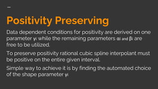
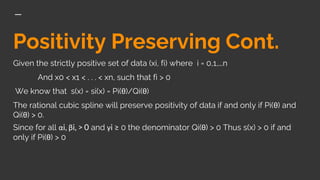
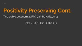
Linear interpolation, cubic interpolation, rational cubic spline with positivity, monotony and convexity preserving technique and shape preserving interpolation.
2. Linear Interpolation
Linear Interpolation is a way of curve fitting the
points by using linear polynomial such as the
equation of the line. This is just similar to joining
points by drawing a line between the two points in
the dataset.
3. Cubic Spline
A cubic spline is a spline constructed of piecewise
third-order polynomials which pass through a set
of control points.
6. Cubic Spline
➔ WEAKNESS
If the given data is positive
cubic spline may give some
negative values along the
whole interval.
7. Cubic Spline
➔ WEAKNESS
For some application
negativity is unacceptable.
Eg: Wind Speed, Solar
energy and rainfall received
are always having positive
values.
10. Fritsch and Carlson
Used cubic spline interpolation by modifying the first
derivative values in which shape violation is found.
11. Butt and Brodlie
Used cubic spline interpolation to preserve the positivity
and convexity of the finite data by inserting extra knots in
the interval.
12. Drawbacks
Did not give any extra freedom to the user in controlling the
final shape of the interpolating curves.
Their method require the modification of the first derivative
parameters.
13. C2 Rational Cubic
Spline Interpolant
It is interpolation with cubic numerator and quadratic denominator which
is used for shape preserving interpolation for positive data.
It has three parameters αi, βi, γi
Sufficient condition for positivity are derived on one parameter γi
αi and βi are free parameters that can be used to change the final shape
of the resulting interpolating curves.
14. Features
It works for both equally and unequally spaced data.
It doesn’t require any knots insertion.
Provides greater flexibility to the user in controlling the final shape of the
interpolating curves.
15. C2 Rational Cubic
Spline Interpolant
Given the set of data points
{(xi, fi), i = 0,1,....n}
such that x0 < x1 < … Xn
Let hi= xi+1 -xi, Δi= (fi+1 -fi)/hi and θ = (x-xi)/hi where 0 ≤ θ ≤ 1
16. C2 Rational Cubic Cont.
Now, cubic spline with three parameters is defined as follows:
Also we can write s(x) = si(x) = Pi(θ)/Qi(θ)s(x) = si(x) = Pi()/Qi()s(x)
= si(x) = Pi()/Qi()s(x) = si(x) = Pi()/Qi()
17. C2 Rational Cubic Cont.
The following conditions will assure that the relational cubic spline
interpolation above has C2 continuity:
18. C2 Rational Cubic Cont.
The required C2 rational cubic spline interpolation with three parameters
has the unknown Aij where j=0,1,2,3 and is given as follows:
The parameters αi, βi > 0, γi ≥ are used to control the final shape of the
interpolating curves.
19. Positivity Preserving
Data dependent conditions for positivity are derived on one
parameter γi while the remaining parameters αi and βi are
free to be utilized.
To preserve positivity rational cubic spline interpolant must
be positive on the entire given interval.
Simple way to achieve it is by finding the automated choice
of the shape parameter γi
20. Positivity Preserving Cont.
Given the strictly positive set of data (xi, fi) where i = 0,1,...n
And x0 < x1 < . . . < xn, such that fi > 0
We know that s(x) = si(x) = Pi(θ)/Qi(θ)
The rational cubic spline will preserve positivity of data if and only if Pi(θ) and
Qi(θ) > 0.
Since for all αi, βi, > 0 and γi ≥ 0 the denominator Qi(θ) > 0 Thus s(x) > 0 if and
only if Pi(θ) > 0