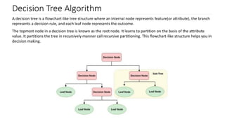
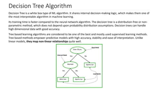
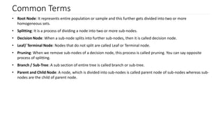
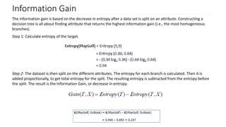
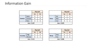
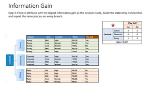
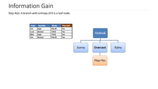
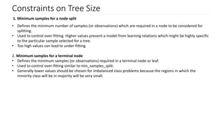
The document discusses decision trees as a key classification technique in machine learning, highlighting their structure, advantages, and common terminology. It explains the algorithm's process for creating a tree by recursively selecting attributes to split data based on measures like information gain and Gini index, which assess the purity of data subsets. Constraints on tree size are also addressed, including minimum samples for node splits, maximum depth, and maximum terminal nodes, essential for managing overfitting.

1. Lesson 17
Classification Techniques – Decision Trees Kush Kulshrestha

2. Decision Tree Algorithm
A decision tree is a flowchart-like tree structure where an internal node represents feature(or attribute), the branch
represents a decision rule, and each leaf node represents the outcome.
The topmost node in a decision tree is known as the root node. It learns to partition on the basis of the attribute
value. It partitions the tree in recursively manner call recursive partitioning. This flowchart-like structure helps you in
decision making.

3. Decision Tree Algorithm
Decision Tree is a white box type of ML algorithm. It shares internal decision-making logic, which makes them one of
the most interpretable algorithm in machine learning.
Its training time is faster compared to the neural network algorithm. The decision tree is a distribution-free or non-
parametric method, which does not depend upon probability distribution assumptions. Decision trees can handle
high dimensional data with good accuracy.
Tree based learning algorithms are considered to be one of the best and mostly used supervised learning methods.
Tree based methods empower predictive models with high accuracy, stability and ease of interpretation. Unlike
linear models, they map non-linear relationships quite well.

4. Common Terms
• Root Node: It represents entire population or sample and this further gets divided into two or more
homogeneous sets.
• Splitting: It is a process of dividing a node into two or more sub-nodes.
• Decision Node: When a sub-node splits into further sub-nodes, then it is called decision node.
• Leaf/ Terminal Node: Nodes that do not split are called Leaf or Terminal node.
• Pruning: When we remove sub-nodes of a decision node, this process is called pruning. You can say opposite
process of splitting.
• Branch / Sub-Tree: A sub section of entire tree is called branch or sub-tree.
• Parent and Child Node: A node, which is divided into sub-nodes is called parent node of sub-nodes whereas sub-
nodes are the child of parent node.

5. Working of the Algo
1. Select the best attribute using Attribute Selection Measures(ASM) to split the records.
2. Make that attribute a decision node and breaks the dataset into smaller subsets.
3. Starts tree building by repeating this process recursively for each child until one of the condition will match:
1. All the tuples belong to the same attribute value.
2. There are no more remaining attributes
3. There are no more instances.

6. Attribute Selection Measures
Attribute selection measure is a heuristic for selecting the splitting criterion that partition data into the best possible
manner.
It is also known as splitting rules because it helps us to determine breakpoints for tuples on a given node.
ASM provides a rank to each feature(or attribute) by explaining the given dataset. Best score attribute will be
selected as a splitting attribute.
Most popular selection measures are Information Gain, Gini Index.

7. Information Gain
• Shannon invented the concept of entropy, which measures the impurity of the input set. In physics and
mathematics, entropy referred as the randomness or the impurity in the system. In information theory, it refers to
the impurity in a group of examples.
• Information gain is the decrease in entropy.
• Information gain computes the difference between entropy before split and average entropy after split of the
dataset based on given attribute values.
• ID3 (Iterative Dichotomiser) decision tree algorithm uses information gain.
• Less impure node requires less information to describe it. And, more impure node requires more information.
Information theory is a measure to define this degree of disorganization in a system known as Entropy.
• If the sample is completely homogeneous, then the entropy is zero and if the sample is an equally divided (50% —
50%), it has entropy of one.
• Entropy can be calculated using formula:- Entropy = -p log2 p — q log2q,
Where p and q is probability of success and failure respectively in that node.
• Entropy is also used with categorical target variable. It chooses the split which has lowest entropy compared to
parent node and other splits. The lesser the entropy, the better it is.

8. Information Gain
To build a decision tree, we need to calculate two types of entropy using frequency tables as follows:
1) Entropy using the frequency table of one attribute
2) Entropy using the frequency table of two attributes

9. Information Gain
1) Entropy using the frequency table of one attribute

10. Information Gain
2. Entropy using the frequency table of two attributes

11. Information Gain
The information gain is based on the decrease in entropy after a data-set is split on an attribute. Constructing a
decision tree is all about finding attribute that returns the highest information gain (i.e., the most homogeneous
branches).
Step 1: Calculate entropy of the target.
Step 2: The dataset is then split on the different attributes. The entropy for each branch is calculated. Then it is
added proportionally, to get total entropy for the split. The resulting entropy is subtracted from the entropy before
the split. The result is the Information Gain, or decrease in entropy.

12. Information Gain

13. Information Gain
Step 3: Choose attribute with the largest information gain as the decision node, divide the dataset by its branches
and repeat the same process on every branch.

14. Information Gain
Step 4(a): A branch with entropy of 0 is a leaf node.

15. Information Gain
Step 4(b): A branch with entropy more than 0 needs further splitting.

16. Gini Index
Steps to Calculate Gini for a split:
1. Calculate Gini for sub-nodes, using formula sum of square of probability for success and failure (p²+q²).
2. Calculate Gini for split using weighted Gini score of each node of that split.
Referring to example where we want to segregate the students based on target variable ( playing cricket or not ). In
the snapshot below, we split the population using two input variables Gender and Class. Now, I want to identify
which split is producing more homogeneous sub-nodes using Gini index.

17. Gini Index
Split on Gender:
• Gini for sub-node Female = (0.2)*(0.2)+(0.8)*(0.8)=0.68
• Gini for sub-node Male = (0.65)*(0.65)+(0.35)*(0.35)=0.55
• Weighted Gini for Split Gender = (10/30)*0.68+(20/30)*0.55 = 0.59

18. Gini Index
Similar for Split on Class:
• Gini for sub-node Class IX = (0.43)*(0.43)+(0.57)*(0.57)=0.51
• Gini for sub-node Class X = (0.56)*(0.56)+(0.44)*(0.44)=0.51
• Weighted Gini for Split Class = (14/30)*0.51+(16/30)*0.51 = 0.51

19. Gini Index
Gini score for split on Gender: 0.59
Gini score on the split on Class: 0.51
Above, you can see that Gini score for Split on Gender is higher than Split on Class, hence, the node split will take
place on Gender.

20. Constraints on Tree Size
1. Minimum samples for a node split
• Defines the minimum number of samples (or observations) which are required in a node to be considered for
splitting.
• Used to control over-fitting. Higher values prevent a model from learning relations which might be highly specific
to the particular sample selected for a tree.
• Too high values can lead to under-fitting.
2. Minimum samples for a terminal node
• Defines the minimum samples (or observations) required in a terminal node or leaf.
• Used to control over-fitting similar to min_samples_split.
• Generally lower values should be chosen for imbalanced class problems because the regions in which the
minority class will be in majority will be very small.

21. Constraints on Tree Size
3. Maximum depth of tree
• The maximum depth of a tree.
• Used to control over-fitting as higher depth will allow model to learn relations very specific to a particular sample.
4. Maximum number of terminal nodes
• The maximum number of terminal nodes or leaves in a tree.
• Can be defined in place of max_depth. Since binary trees are created, a depth of ’n’ would produce a maximum of
2^n leaves.
5. Maximum features to consider for split
• The number of features to consider while searching for a best split. These will be randomly selected.
• As a thumb-rule, square root of the total number of features works great but we should check upto 30–40% of
the total number of features.
• Higher values can lead to over-fitting but depends on case to case.