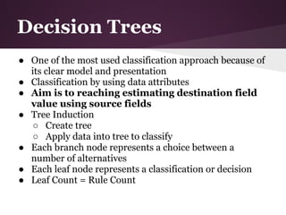
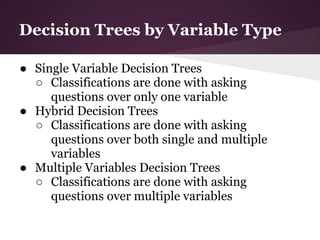
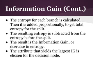
![ID3 Algorithm Steps
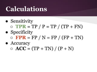
function ID3 (R: a set of non-categorical attributes,
C: the categorical attribute,
S: a training set) returns a decision tree;
begin
If S is empty, return a single node with value Failure;
If S consists of records all with the same value for
the categorical attribute,
return a single node with that value;
If R is empty, then return a single node with as value
the most frequent of the values of the categorical attribute
that are found in records of S; [note that then there
will be errors, that is, records that will be improperly
classified];
Let D be the attribute with largest Gain( D,S)
among attributes in R;
Let {dj| j=1,2, .., m} be the values of attribute D;
Let {Sj| j=1,2, .., m} be the subsets of S consisting
respectively of records with value dj for attribute D;
Return a tree with root labeled D and arcs labeled
d1, d2, .., dm going respectively to the trees
ID3(R-{D}, C, S1), ID3(R-{D}, C, S2), .., ID3(R-{D}, C, Sm);
end ID3;](https://image.slidesharecdn.com/id3algorithmrocanalysis-121101120125-phpapp02/85/ID3-Algorithm-ROC-Analysis-22-320.jpg)
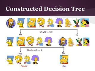
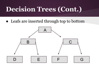
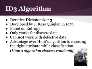
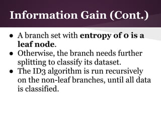
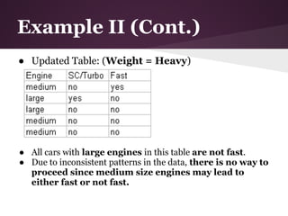
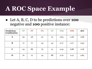
![Example II (Cont.)
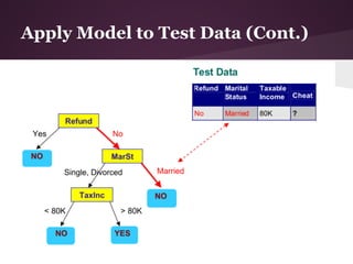
Information Gain over Engine
● Engine: 6 small, 5 medium, 4 large
● 3 values for attribute engine, so we need 3 entropy
calculations
● small: 5 no, 1 yes
○ IGsmall = -(5/6)log2(5/6)-(1/6)log2(1/6) = ~0.65
● medium: 3 no, 2 yes
○ IGmedium = -(3/5)log2(3/5)-(2/5)log2(2/5) = ~0.97
● large: 2 no, 2 yes
○ IGlarge = 1 (evenly distributed subset)
=> IGEngine = IE(S) – [(6/15)*IGsmall + (5/15)*IGmedium +
(4/15)*Ilarge]
= IGEngine = 0.918 – 0.85 = 0.068](https://image.slidesharecdn.com/id3algorithmrocanalysis-121101120125-phpapp02/85/ID3-Algorithm-ROC-Analysis-33-320.jpg)
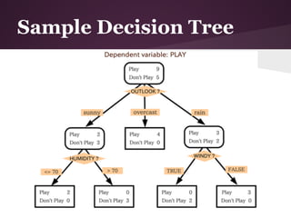
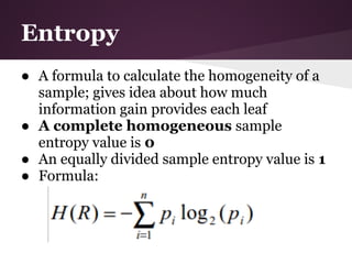
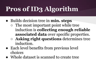
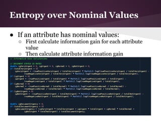
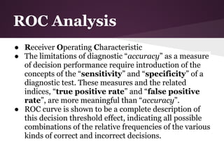
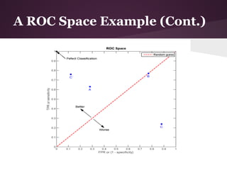
![Example II (Cont.)
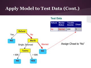
Information Gain over SC/Turbo
● SC/Turbo: 4 yes, 11 no
● 2 values for attribute SC/Turbo, so we need 2 entropy
calculations
● yes: 2 yes, 2 no
○ IGturbo = 1 (evenly distributed subset)
● no: 3 yes, 8 no
○ IGnoturbo = -(3/11)log2(3/11)-(8/11)log2(8/11) = ~0.84
IGturbo = IE(S) – [(4/15)*IGturbo + (11/15)*IGnoturbo]
IGturbo = 0.918 – 0.886 = 0.032](https://image.slidesharecdn.com/id3algorithmrocanalysis-121101120125-phpapp02/85/ID3-Algorithm-ROC-Analysis-34-320.jpg)
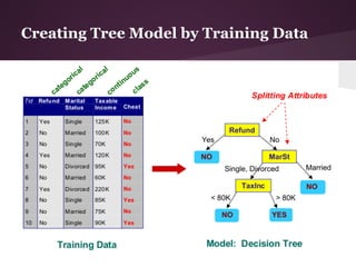
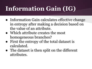
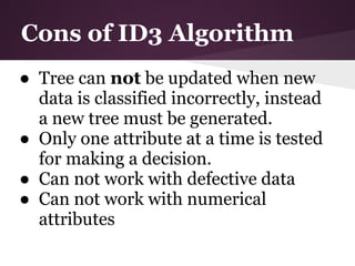
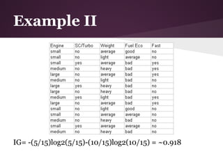
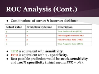
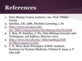
![Example II (Cont.)
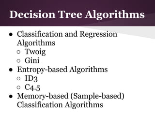
Information Gain over Weight
● Weight: 6 Average, 4 Light, 5 Heavy
● 3 values for attribute weight, so we need 3 entropy
calculations
● average: 3 no, 3 yes
○ IGaverage = 1 (evenly distributed subset)
● light: 3 no, 1 yes
○ IGlight = -(3/4)log2(3/4)-(1/4)log2(1/4) = ~0.81
● heavy: 4 no, 1 yes
○ IGheavy = -(4/5)log2(4/5)-(1/5)log2(1/5) = ~0.72
IGWeight = IE(S) – [(6/15)*IGaverage + (4/15)*IGlight + (5/15)*IGheavy]
IGWeight = 0.918 – 0.856 = 0.062](https://image.slidesharecdn.com/id3algorithmrocanalysis-121101120125-phpapp02/85/ID3-Algorithm-ROC-Analysis-35-320.jpg)
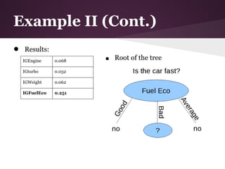
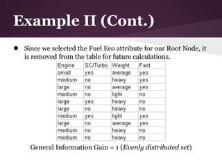
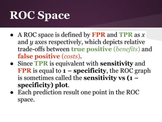
![Example II (Cont.)
Information Gain over Full Eco
● Fuel Economy: 2 good, 3 average, 10 bad
● 3 values for attribute Fuel Eco, so we need 3 entropy
calculations
● good: 0 yes, 2 no
○ IGgood = 0 (no variability)
● average: 0 yes, 3 no
○ IGaverage = 0 (no variability)
● bad: 5 yes, 5 no
○ IGbad = 1 (evenly distributed subset)
We can omit calculations for good and average since they always
end up not fast.
IGFuelEco = IE(S) – [(10/15)*IGbad]
IGFuelEco = 0.918 – 0.667 = 0.251](https://image.slidesharecdn.com/id3algorithmrocanalysis-121101120125-phpapp02/85/ID3-Algorithm-ROC-Analysis-36-320.jpg)
![Example II (Cont.)
Information Gain over Engine
● Engine: 1 small, 5 medium, 4 large
● 3 values for attribute engine, so we need 3 entropy calculations
● small: 1 yes, 0 no
○ IGsmall = 0 (no variability)
● medium: 2 yes, 3 no
○ IGmedium = -(2/5)log2(2/5)-(3/5)log2(3/5) = ~0.97
● large: 2 no, 2 yes
○ IGlarge = 1 (evenly distributed subset)
IGEngine = IE(SFuelEco) – (5/10)*IGmedium + (4/10)*IGlarge]
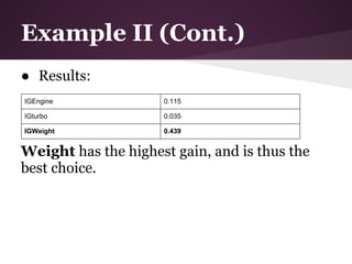
IGEngine = 1 – 0.885 = 0.115](https://image.slidesharecdn.com/id3algorithmrocanalysis-121101120125-phpapp02/85/ID3-Algorithm-ROC-Analysis-39-320.jpg)
![Example II (Cont.)
Information Gain over SC/Turbo
● SC/Turbo: 3 yes, 7 no
● 2 values for attribute SC/Turbo, so we need 2 entropy calculations
● yes: 2 yes, 1 no
○ IGturbo = -(2/3)log2(2/3)-(1/3)log2(1/3) = ~0.84
● no: 3 yes, 4 no
○ IGnoturbo = -(3/7)log2(3/7)-(4/7)log2(4/7) = ~0.84
IGturbo = IE(SFuelEco) – [(3/10)*IGturbo + (7/10)*IGnoturbo]
IGturbo = 1 – 0.965 = 0.035](https://image.slidesharecdn.com/id3algorithmrocanalysis-121101120125-phpapp02/85/ID3-Algorithm-ROC-Analysis-40-320.jpg)
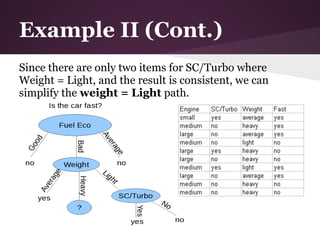
![Example II (Cont.)
Information Gain over Weight
● Weight: 3 average, 5 heavy, 2 light
● 3 values for attribute weight, so we need 3 entropy calculations
● average: 3 yes, 0 no
○ IGaverage = 0 (no variability)
● heavy: 1 yes, 4 no
○ IGheavy = -(1/5)log2(1/5)-(4/5)log2(4/5) = ~0.72
● light: 1 yes, 1 no
○ IlGight = 1 (evenly distributed subset)
IGEngine = IE(SFuel Eco) – [(5/10)*IGheavy+(2/10)*IGlight]
IGEngine = 1 – 0.561 = 0.439](https://image.slidesharecdn.com/id3algorithmrocanalysis-121101120125-phpapp02/85/ID3-Algorithm-ROC-Analysis-41-320.jpg)

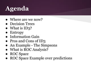
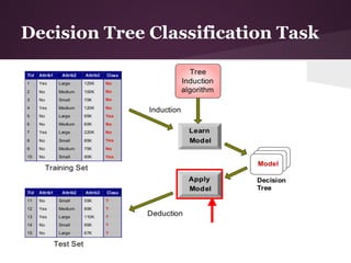
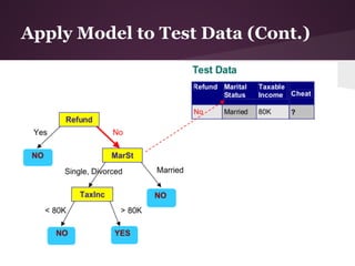
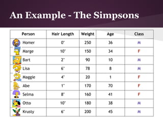
The document discusses decision trees and the ID3 algorithm. It provides an overview of decision trees, describing their structure and how they are used for classification. It then explains the ID3 algorithm, which builds decision trees based on entropy and information gain. The key steps of ID3 are outlined, including calculating entropy and information gain to select the best attributes to split the data on at each node. Pros and cons of ID3 are also summarized. An example applying ID3 to classify characters from The Simpsons is shown.


![Ch 9-2.Machine Learning: Symbol-based[new]](https://cdn.slidesharecdn.com/ss_thumbnails/ch-92machine-learning-symbolbasednew4415-thumbnail.jpg?width=640&height=640&fit=bounds)