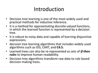
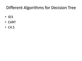
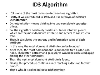
This document discusses decision tree learning algorithms. It begins with an introduction to decision trees, noting that they are widely used for inductive inference and represent learned functions as decision trees. It then discusses appropriate problems for decision tree learning, including instances represented by attribute-value pairs and discrete output values. The document provides examples of different decision tree algorithms like ID3, CART and C4.5 and explains the ID3 algorithm in detail. It also discusses concepts like entropy, information gain and using these measures to determine the best attribute to use at each node in growing the decision tree.

1. Decision Tree Learning

2. Introduction
• Decision tree learning is one of the most widely used and
practical methods for inductive inference.
• It is a method for approximating discrete-valued functions,
in which the learned function is represented by a decision
tree.
• It is robust to noisy data and capable of learning disjunctive
expressions.
• decision tree learning algorithms that includes widely used
algorithms such as ID3, CART, and C4.5.
• Learned trees can also be re-represented as sets of if-then
rules to improve human readability.
• Decision tree algorithms transform raw data to rule based
decision making trees.

3. DECISION TREE REPRESENTATION

5. APPROPRIATE PROBLEMS FOR
DECISION TREE LEARNING
• Instances are represented by attribute-value pairs.
Instances are described by a fixed set of attributes (e.g.,
Temperature) and their values (e.g., Hot, Mild, Cold)
• The target function has discrete output values. assigns a
Boolean classification (e.g., yes or no) to each example.
• Disjunctive descriptions may be required.
• The training data may contain errors. Decision tree
learning methods are robust to errors, both errors in
classifications of the training examples and errors in the
attribute values that describe these examples.
• The training data may contain missing attribute values.
Decision tree methods can be used even when some
training examples have unknown values.

6. Example

7. Different Algorithms for Decision Tree
• ID3
• CART
• C4.5

8. ID3 Algorithm
• ID3 is one of the most common decision tree algorithm.
• Firstly, It was introduced in 1986 and it is acronym of Iterative
Dichotomiser.
• Dichotomisation means dividing into two completely opposite
things.
• So, the algorithm iteratively divides attributes into two groups
which are the most dominant attribute and others to construct a
tree.
• Then, it calculates the entropy and information gains of each
attribute.
• In this way, the most dominant attribute can be founded.
• After then, the most dominant one is put on the tree as decision
node. Thereafter, entropy and gain scores would be calculated again
among the other attributes.
• Thus, the next most dominant attribute is found.
• Finally, this procedure continues until reaching a decision for that
branch.
• That’s why, it is called Iterative Dichotomiser.

10. Which Attribute Is the Best Classifier?
• What is a good quantitative measure of the
worth of an attribute?
• We will define a statistical property, called
information gain.

11. Entropy and Information Gain
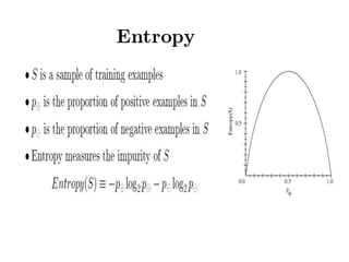
– Entropy(S) = ∑ – p(I) . log2p(I)
– Gain(S, A) = Entropy(S) – ∑ [ p(S|A) . Entropy(S|A) ]

12. Data set

13. Entropy
• We need to calculate the entropy first.
• Decision column consists of 14 instances and includes two
labels: yes and no.
• There are 9 decisions labeled yes, and 5 decisions labeled no.
• Entropy(Decision)
= – p(Yes) . log2p(Yes) – p(No) . log2p(No)
=– (9/14) . log2(9/14) – (5/14) . log2(5/14)
=0.940
• Now, we need to find the most dominant factor for decision.

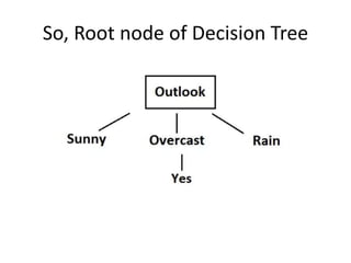
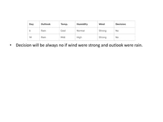
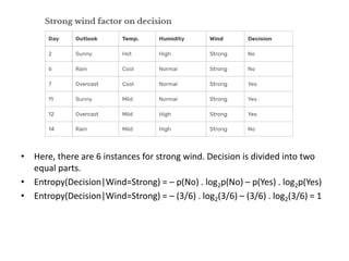
14. Wind factor on decision
• Gain(Decision, Wind) = Entropy(Decision) – ∑ [ p(Decision|Wind) . Entropy(Decision|Wind) ]
• Wind attribute has two labels: weak and strong.
• Now, we need to calculate (Decision|Wind=Weak) and (Decision|Wind=Strong) respectively.
• . There are 8 instances for weak wind. Decision of 2 items are no and 6 items are yes.

15. • Entropy(Decision|Wind=Weak) = – p(No) . log2p(No) – p(Yes) . log2p(Yes)
• Entropy(Decision|Wind=Weak) = – (2/8) . log2(2/8) – (6/8) . log2(6/8) = 0.811

16. • Here, there are 6 instances for strong wind. Decision is divided into two
equal parts.
• Entropy(Decision|Wind=Strong) = – p(No) . log2p(No) – p(Yes) . log2p(Yes)
• Entropy(Decision|Wind=Strong) = – (3/6) . log2(3/6) – (3/6) . log2(3/6) = 1

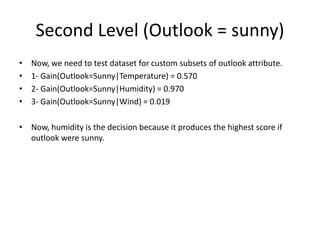
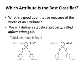
17. • Now compute Gain(Decision, Wind)
• Gain(Decision, Wind) =
Entropy(Decision) – [ p(Decision|Wind=Weak) . Entropy(Decision|Wind=Weak) ]
– [ p(Decision|Wind=Strong) . Entropy(Decision|Wind=Strong) ]
=0.940 – [ (8/14) . 0.811 ] – [ (6/14). 1] = 0.048
• Calculations for wind column is over. Now, we need to apply same calculations
for other columns to find the most dominant factor on decision.

18. Outlook Factor on decision
• outlook attribute has three labels: sunny, rain and overcast.
• Now, we need to calculate (Decision|outlook=sunny) ,
(Decision|outlook=overcast) and (Decision|outlook=rain).

19. • Here, there are 4 instances for outlook=overcast. Decision is consisting only
yes.
• Entropy(Decision|outlook=overcast) = – p(No) . log2p(No) – p(Yes) . log2p(Yes)
• Entropy(Decision|outlook=overcast) = – (0/4) . log2(0/4) – (4/4) . log2(4/4) = 0
• If Entropy is zero, that means data is belonging to single class.
• We can analyse data from table as well, that all examples are falling in ‘yes’
class.

20. • Here, there are 5 instances for outlook=sunny. Decision of 3 items are No and
decision of 2 items are yes.
• Entropy(Decision|outlook=sunny) = – p(No) . log2p(No) – p(Yes) . log2p(Yes)
• Entropy(Decision|outlook=sunny) = – (3/5) . log2(3/5) – (2/5) . log2(2/5) = 0.971

21. • Here, there are 5 instances for outlook=rain. Decision of 2 items are No and
decision of 3 items are yes.
• Entropy(Decision|outlook=rain) = – p(No) . log2p(No) – p(Yes) . log2p(Yes)
• Entropy(Decision|outlook=rain) = – (2/5) . log2(2/5) – (3/5) . log2(3/5) = 0.971

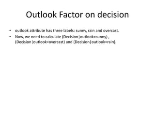
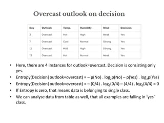
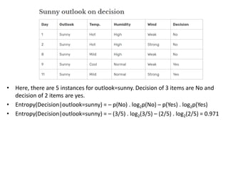
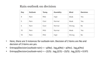
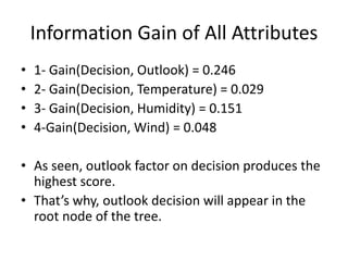
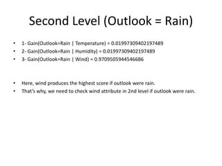
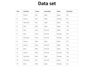
22. • Now compute Gain(Decision, outlook)
• Gain(Decision, outlook) =
Entropy(Decision)
– [ p(Decision|outlook=overcast) . Entropy(Decision|outlook=overcast) ]
– [ p(Decision|outlook=sunny) . Entropy(Decision|outlook=sunny) ]
- [ p(Decision|outlook=rain) . Entropy(Decision|outlook=rain) ]
=0.940 – [ (4/14) . 0 ] – [ (5/14). 0.971] - [ (5/14). 0.971] = 0.246

23. Exercise
• Similarly, compute gain for humidity and temperature

24. Information Gain of All Attributes
• 1- Gain(Decision, Outlook) = 0.246
• 2- Gain(Decision, Temperature) = 0.029
• 3- Gain(Decision, Humidity) = 0.151
• 4-Gain(Decision, Wind) = 0.048
• As seen, outlook factor on decision produces the
highest score.
• That’s why, outlook decision will appear in the
root node of the tree.

25. So, Root node of Decision Tree

26. Second Level (Outlook = sunny)
• Now, we need to test dataset for custom subsets of outlook attribute.
• 1- Gain(Outlook=Sunny|Temperature) = 0.570
• 2- Gain(Outlook=Sunny|Humidity) = 0.970
• 3- Gain(Outlook=Sunny|Wind) = 0.019
• Now, humidity is the decision because it produces the highest score if
outlook were sunny.

27. • At this point, decision will always be no if humidity were high.

28. • On the other hand, decision will always be yes if humidity
were normal

29. Second Level (Outlook = Rain)
• 1- Gain(Outlook=Rain | Temperature) = 0.01997309402197489
• 2- Gain(Outlook=Rain | Humidity) = 0.01997309402197489
• 3- Gain(Outlook=Rain | Wind) = 0.9709505944546686
• Here, wind produces the highest score if outlook were rain.
• That’s why, we need to check wind attribute in 2nd level if outlook were rain.

30. • So, it is revealed that decision will always be yes if wind were
weak and outlook were rain.

31. • Decision will be always no if wind were strong and outlook were rain.

32. Final Decision Tree

33. Exercise