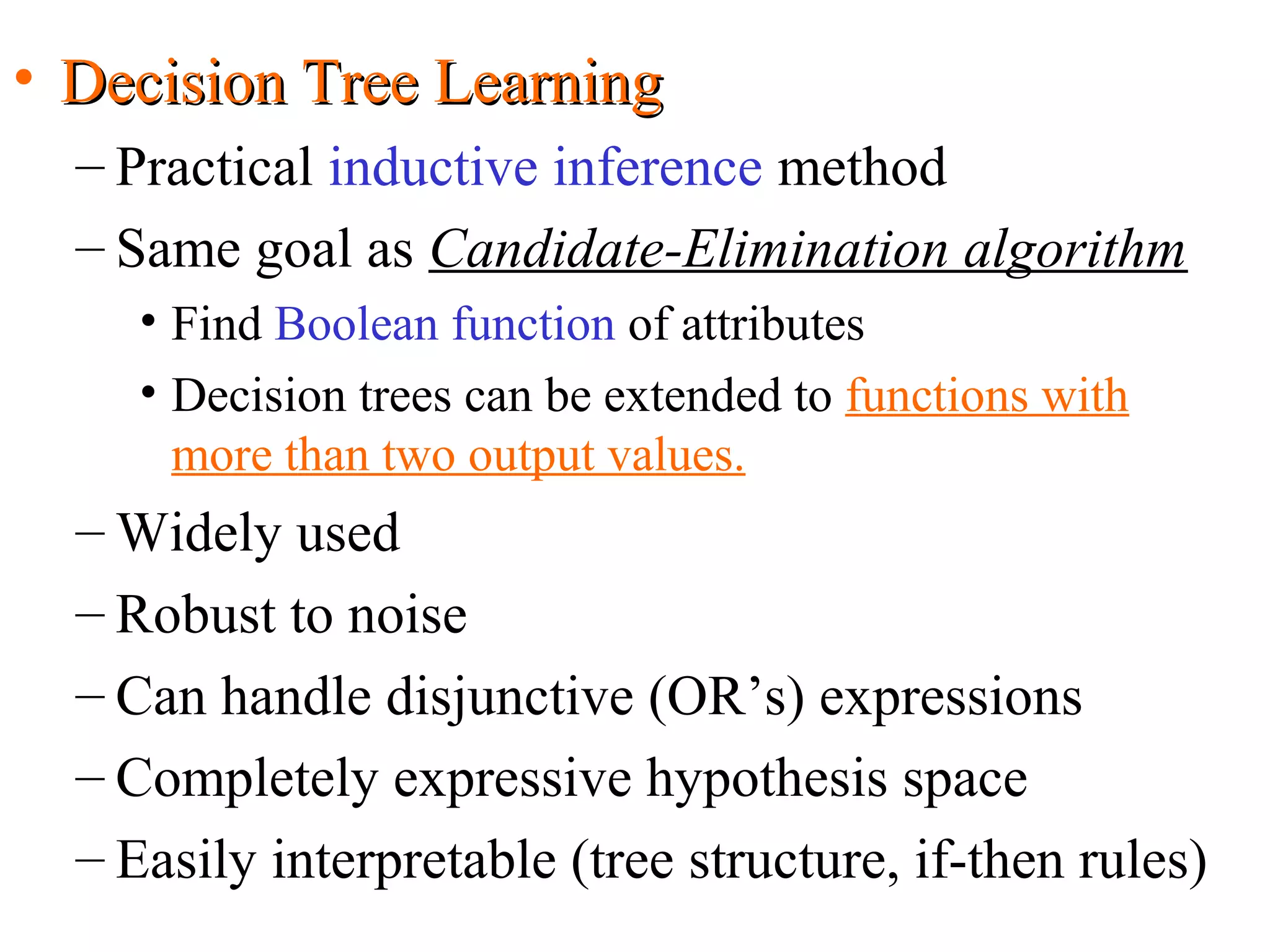
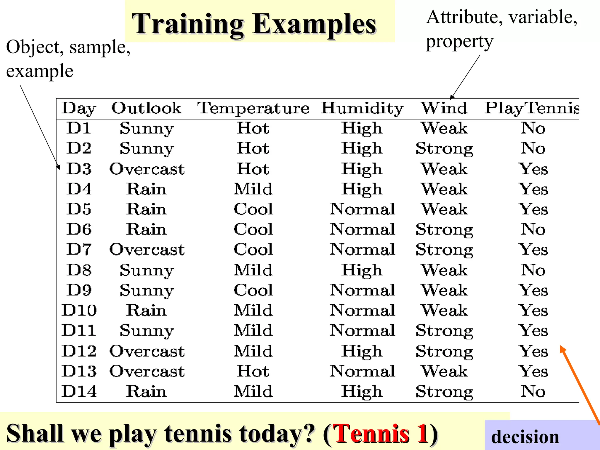
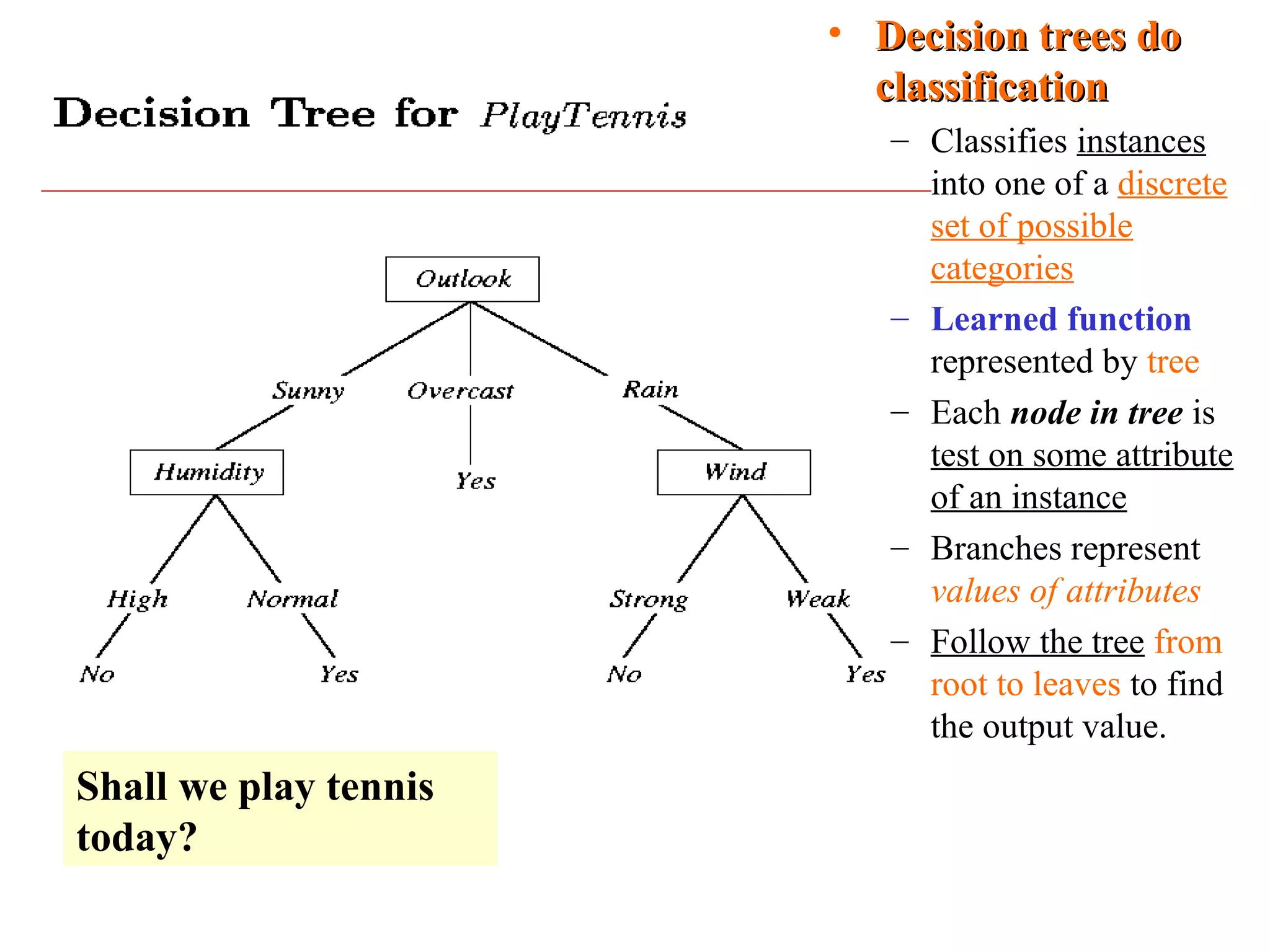
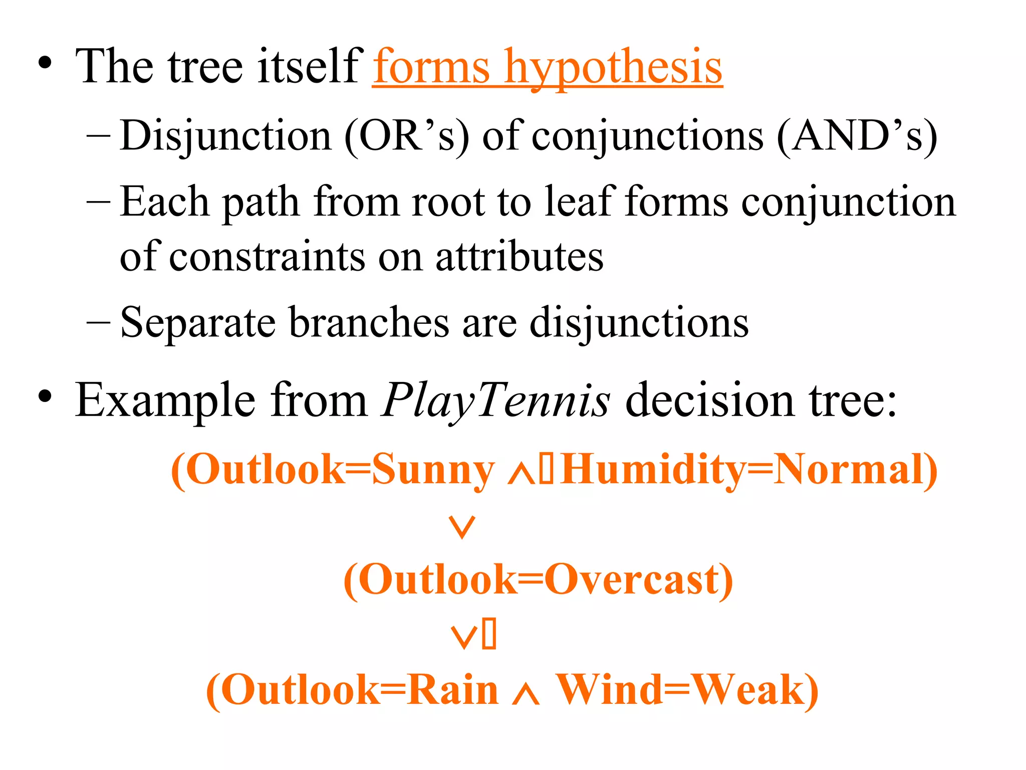
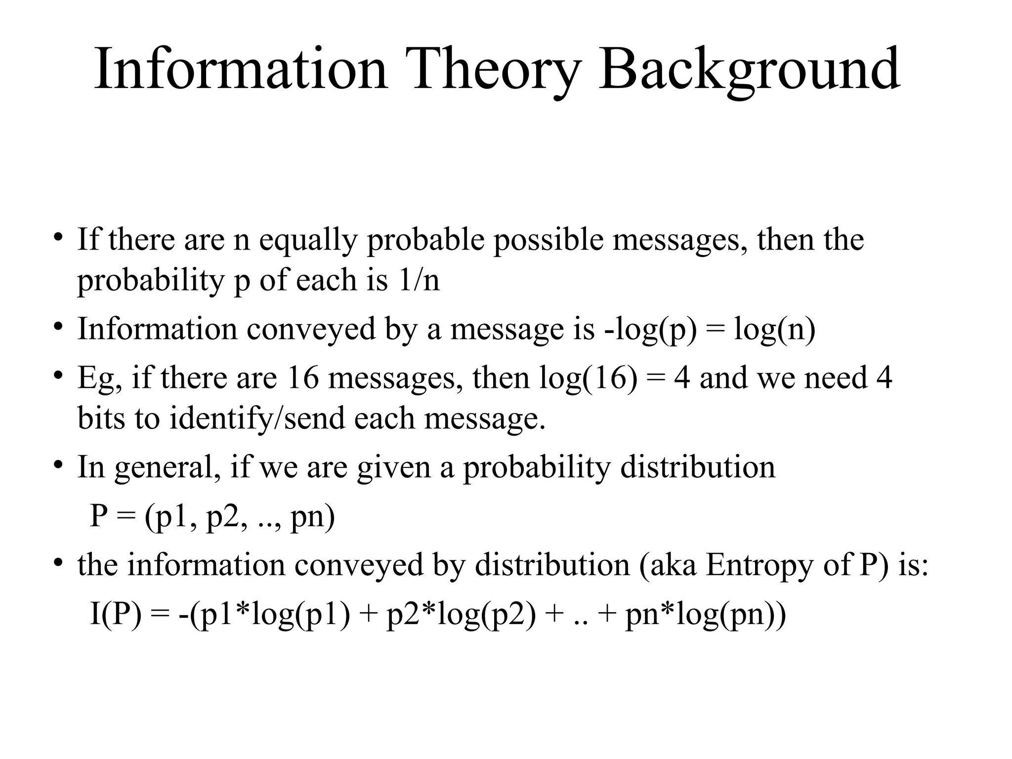
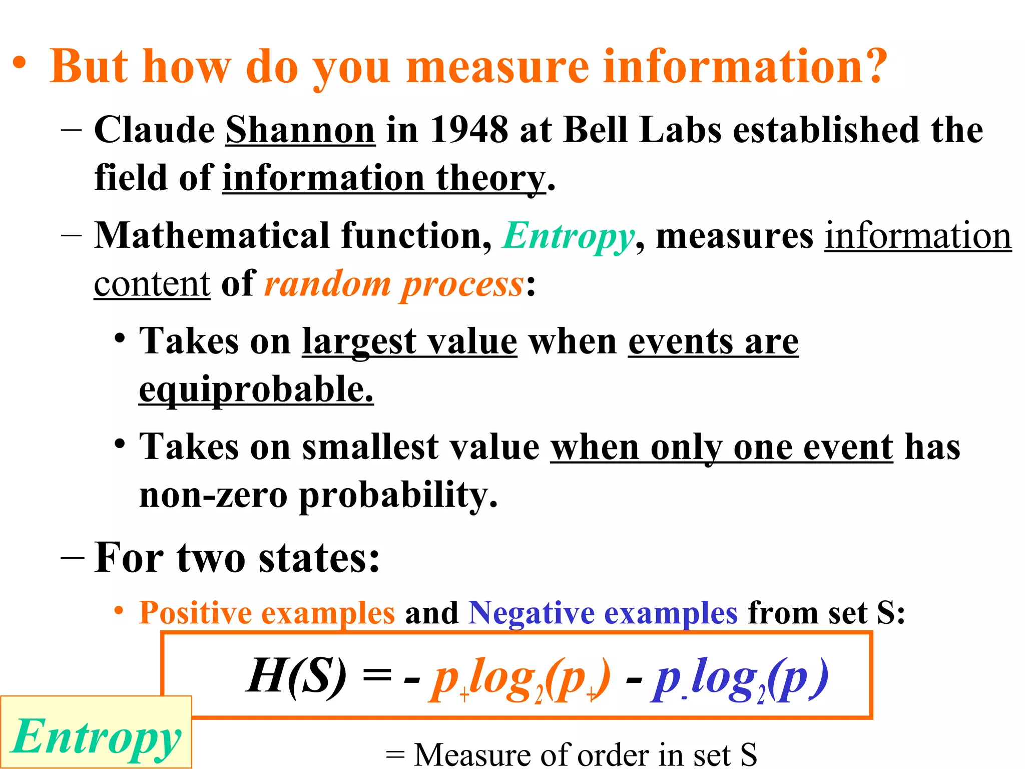
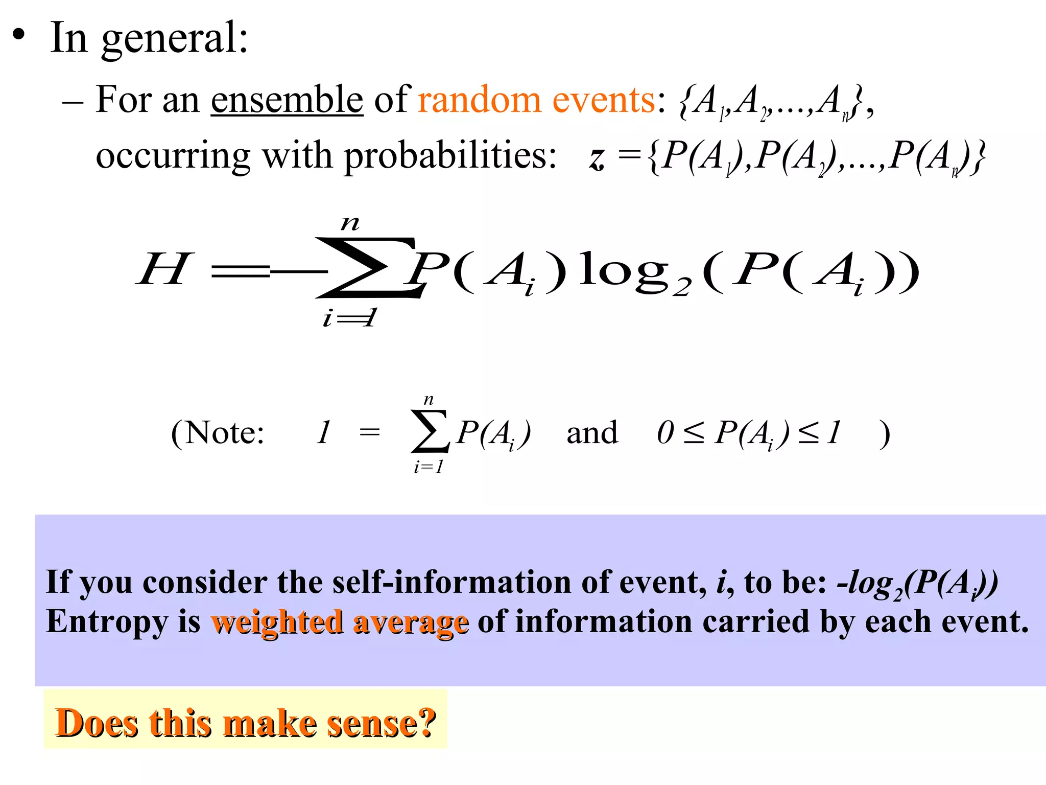
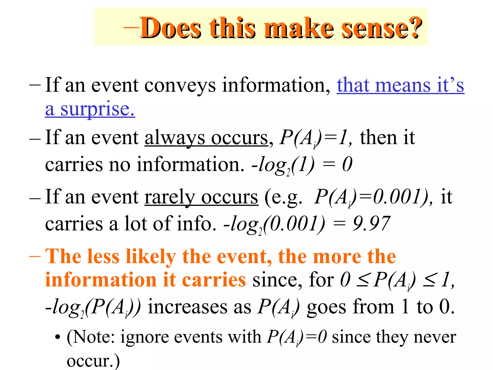
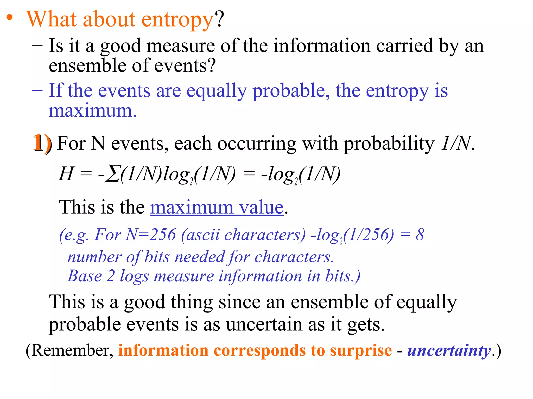
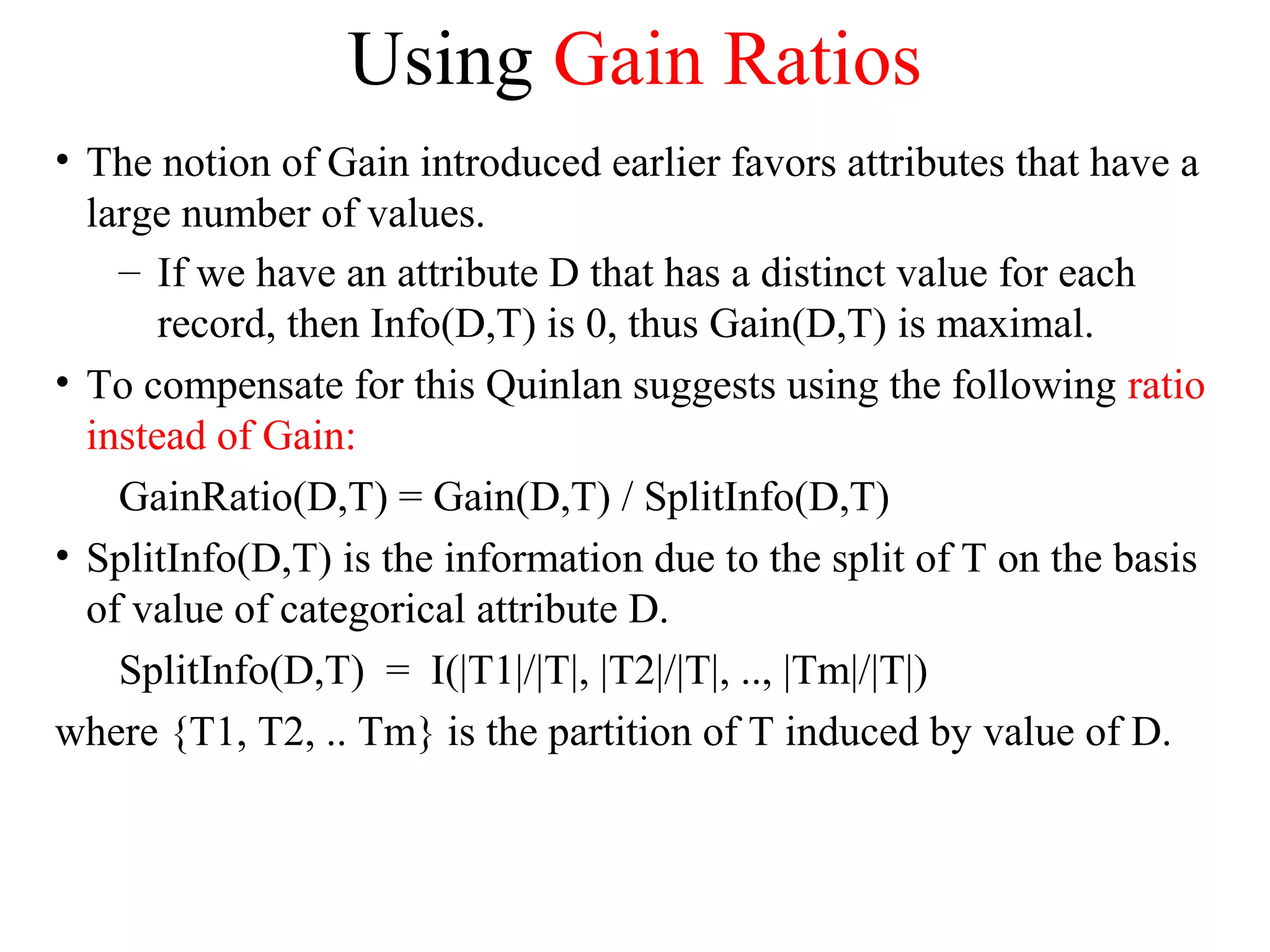
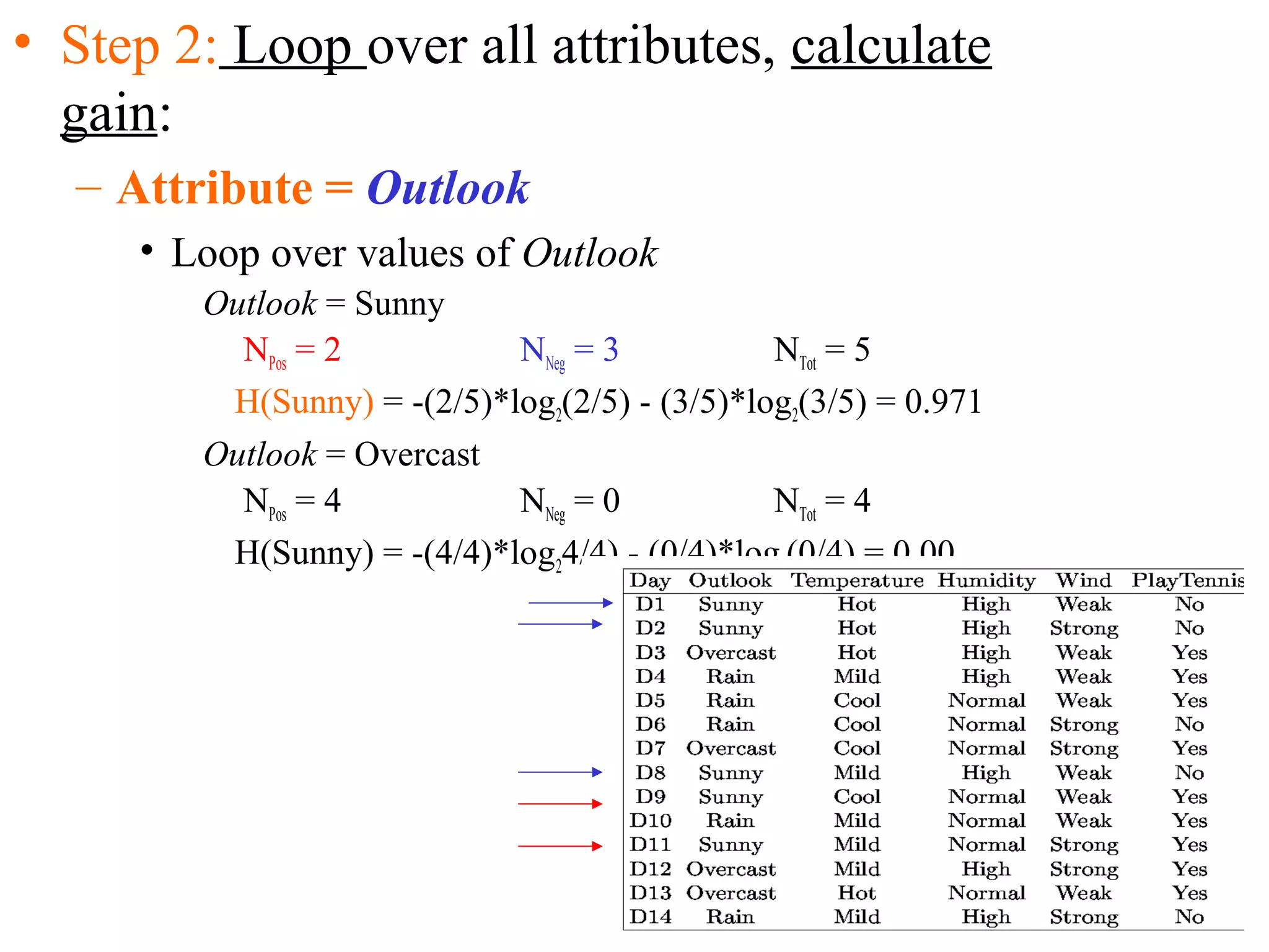
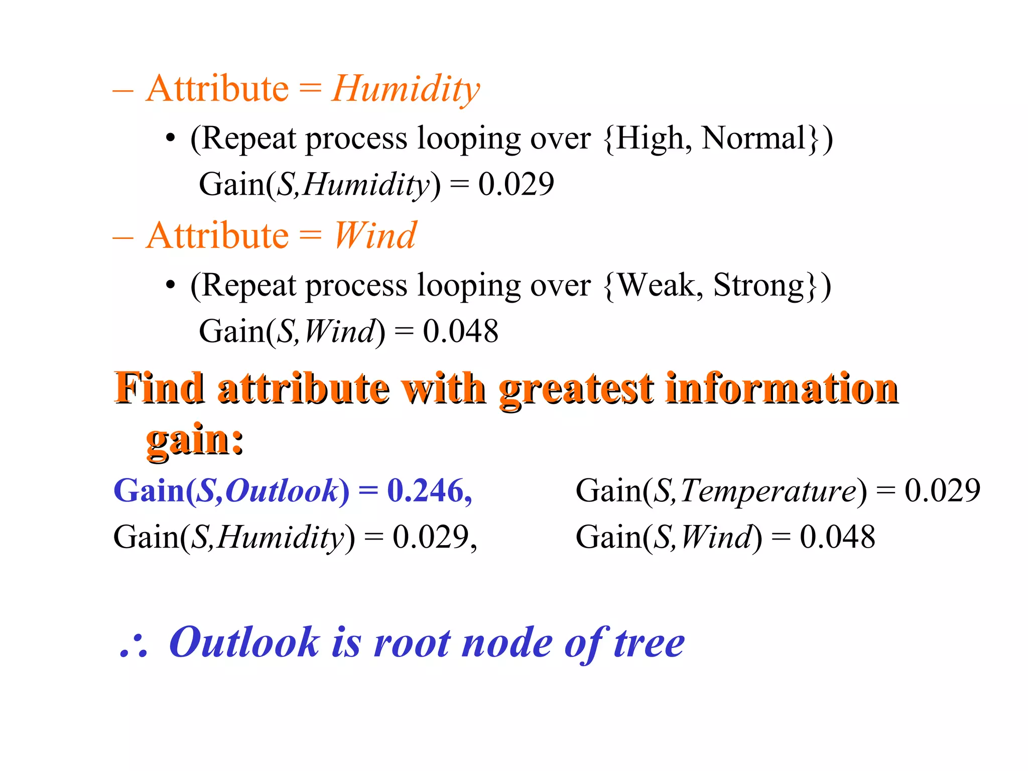
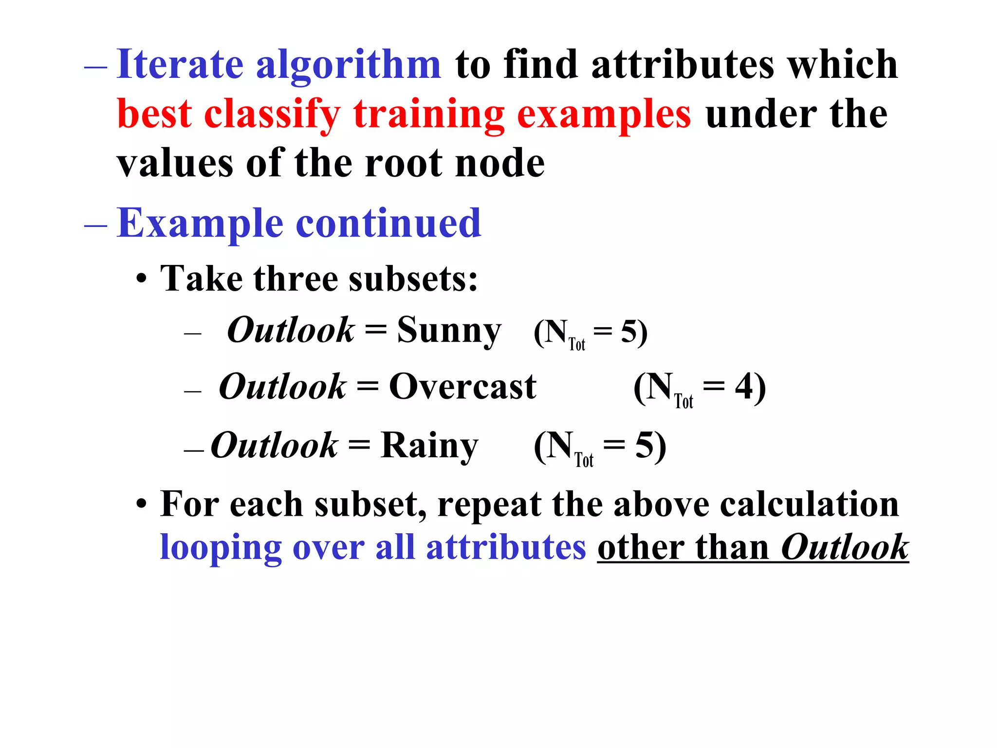
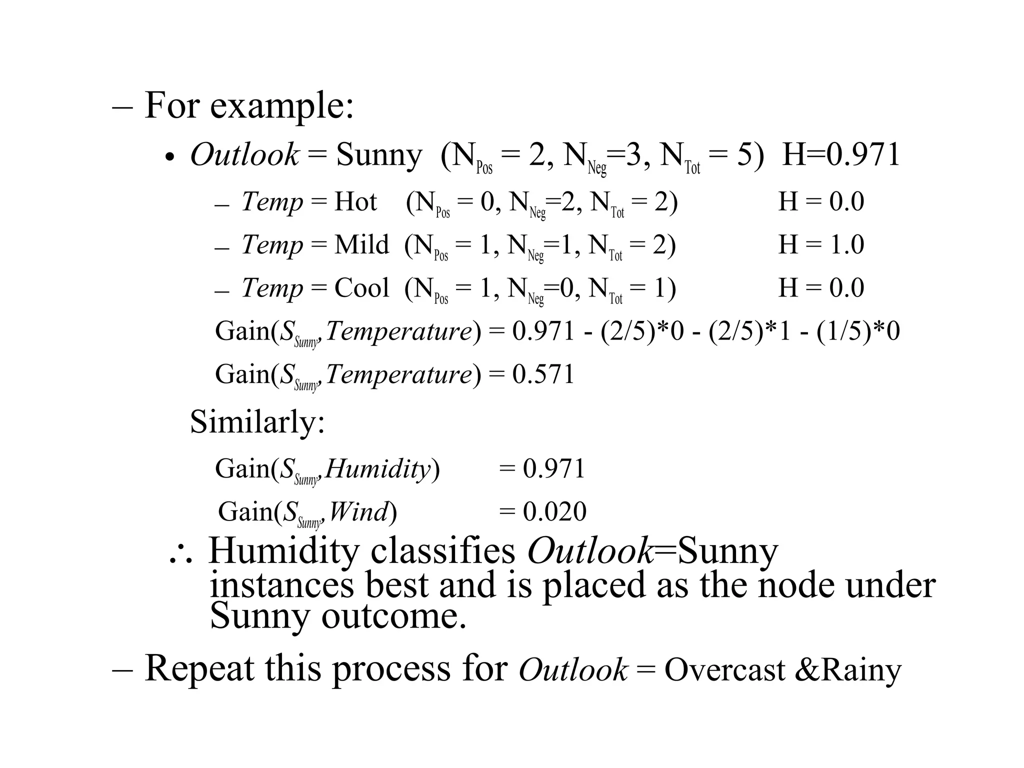
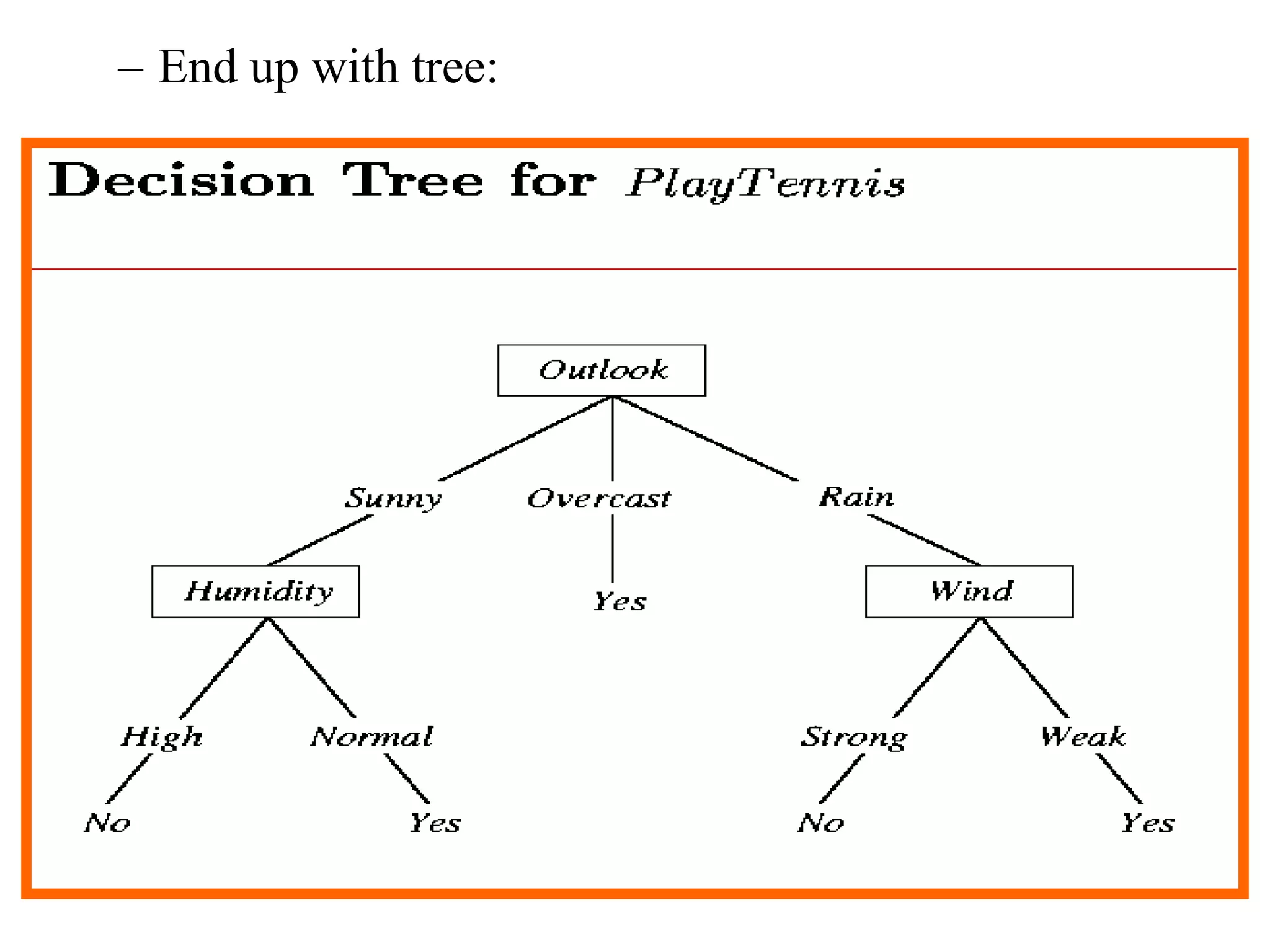
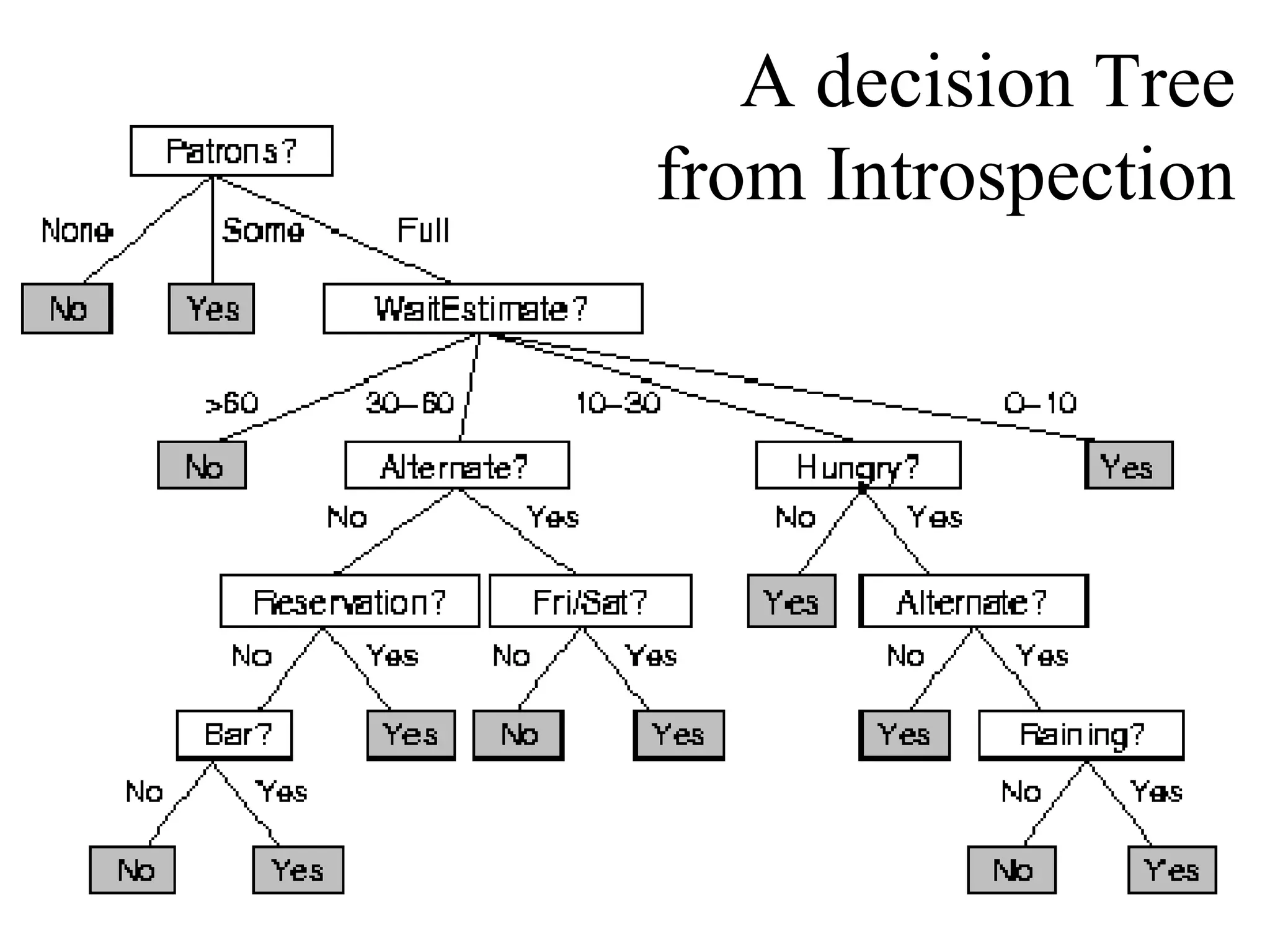
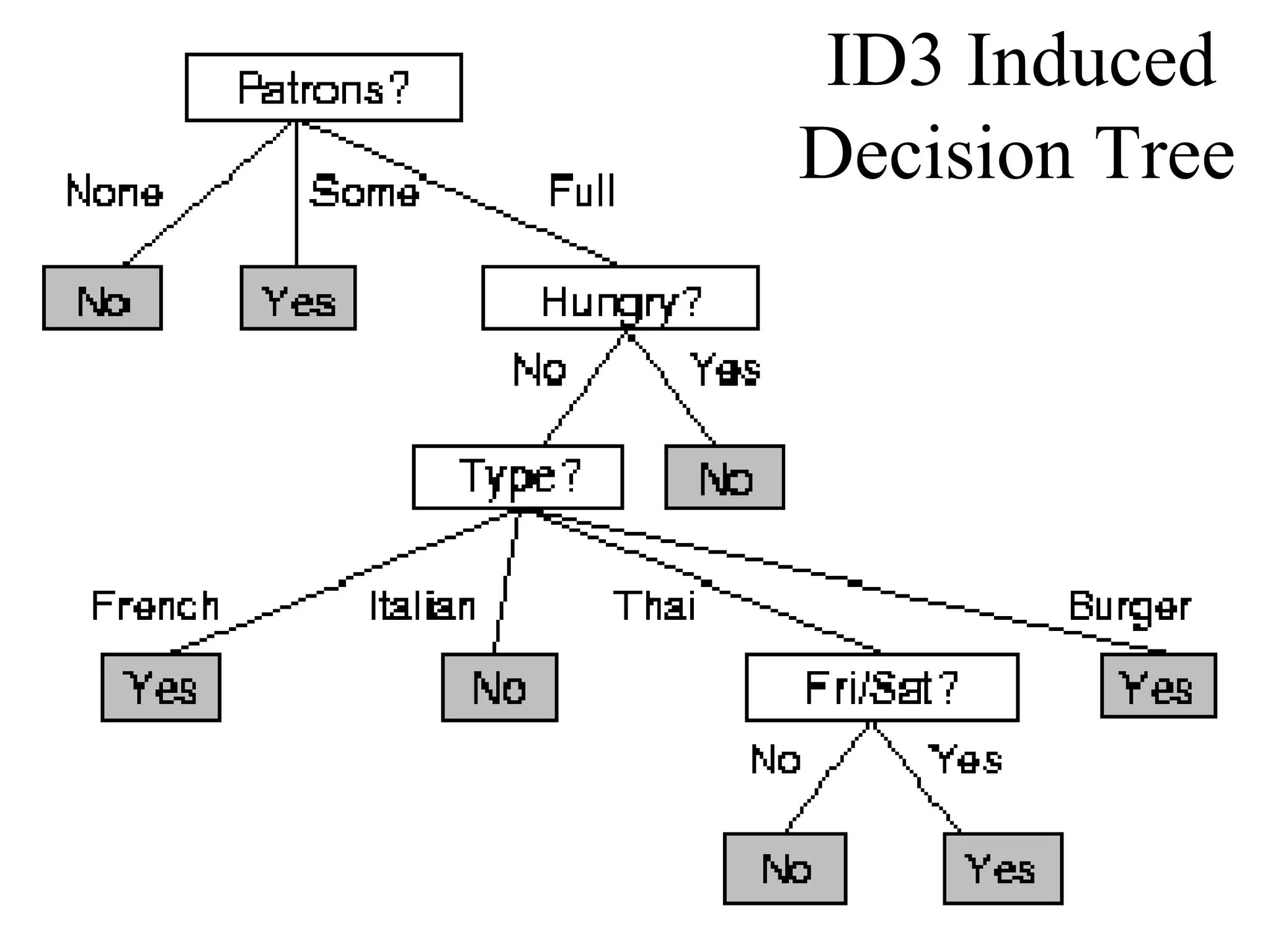
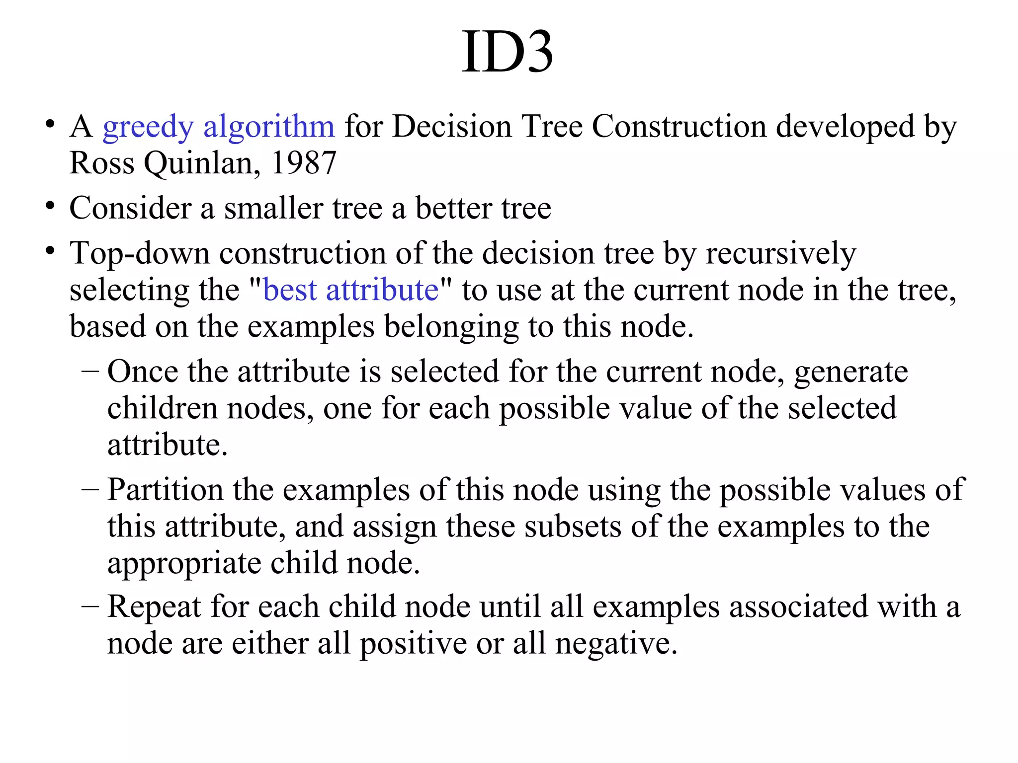
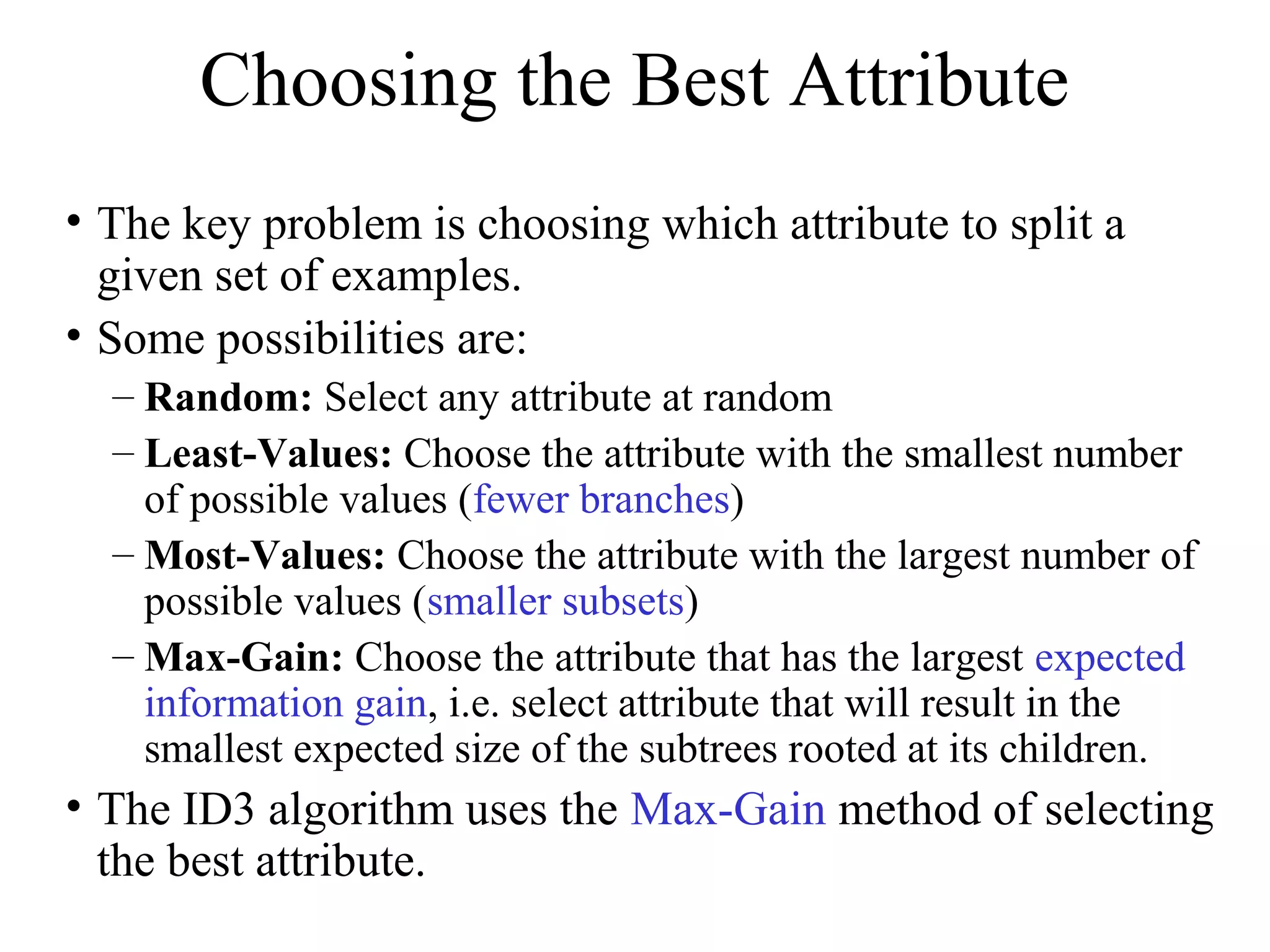
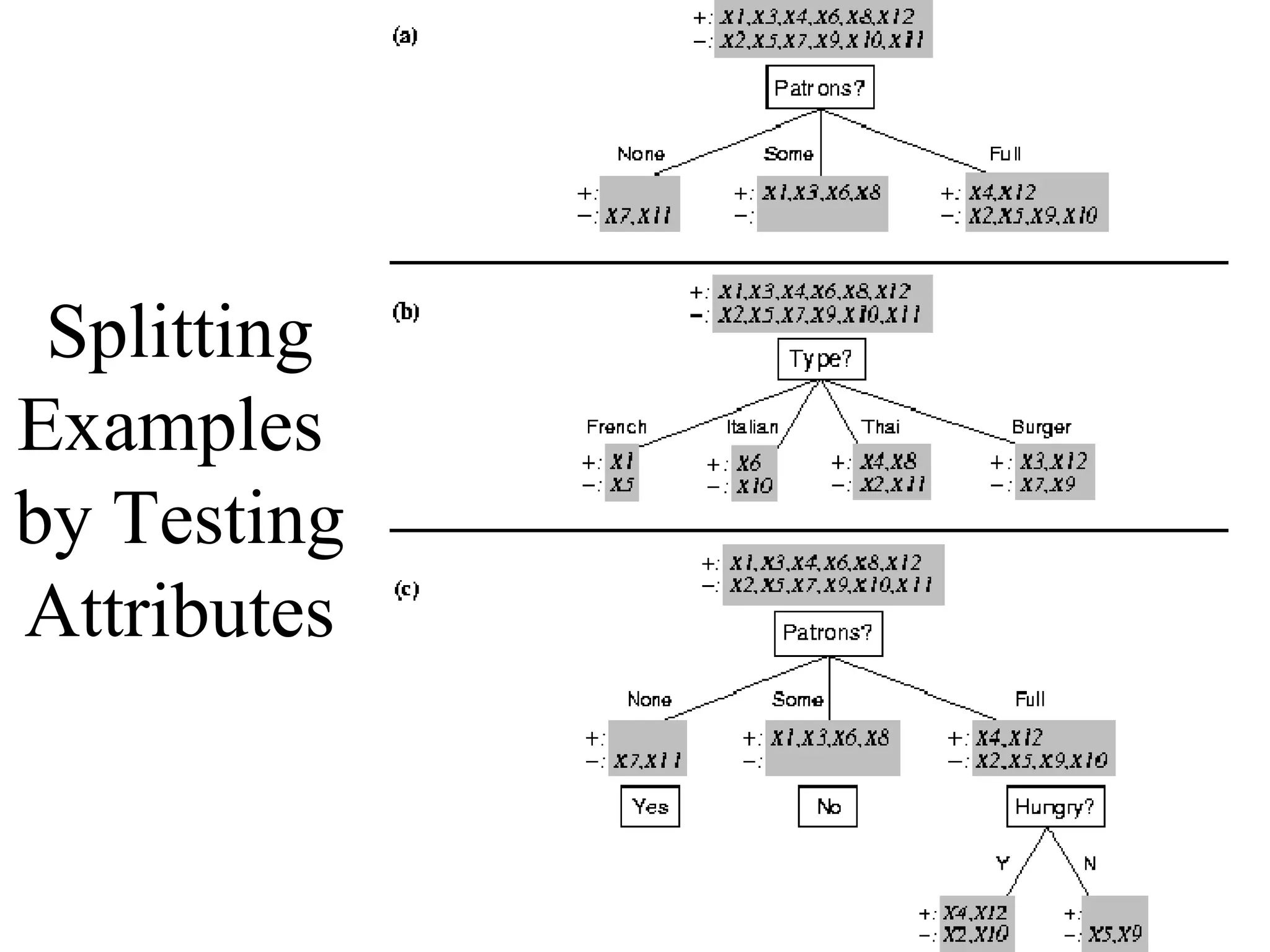
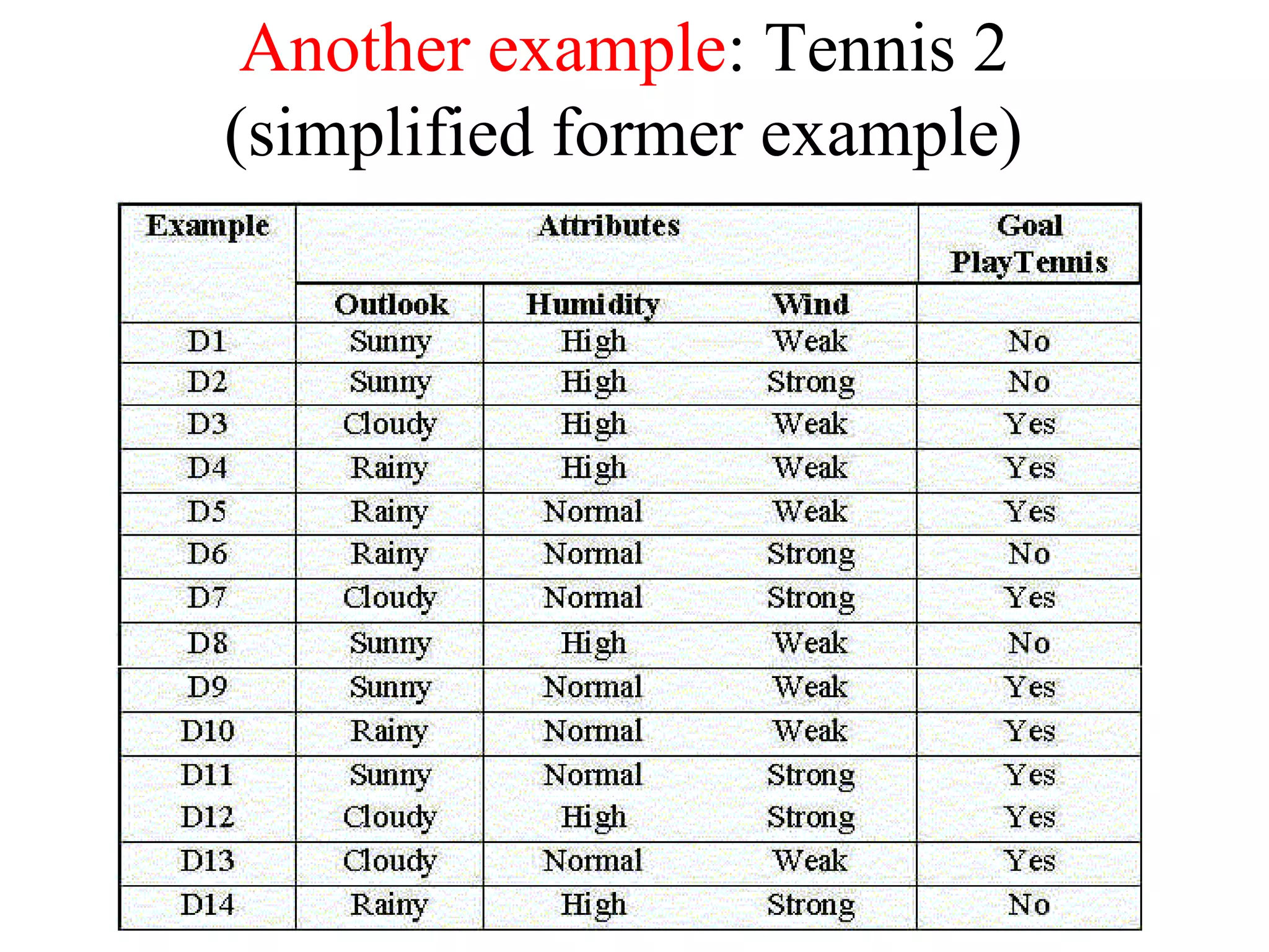
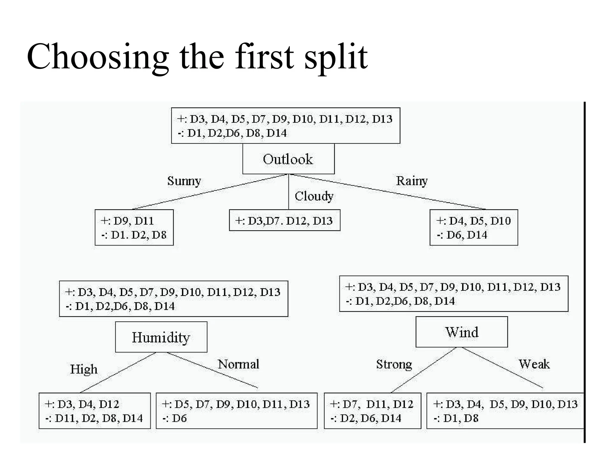
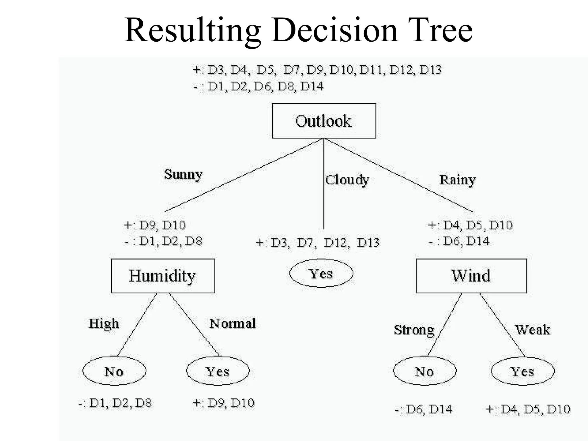
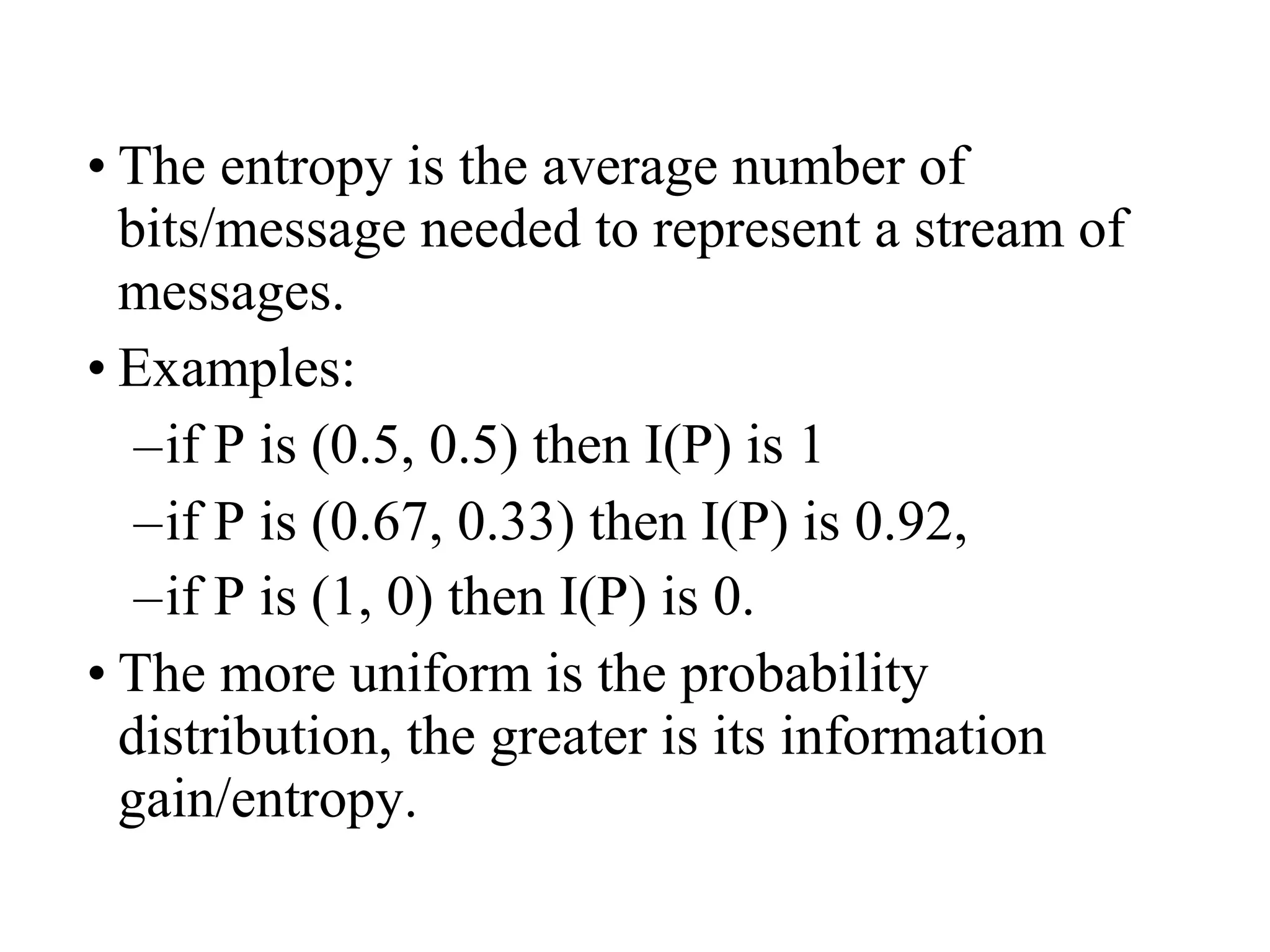
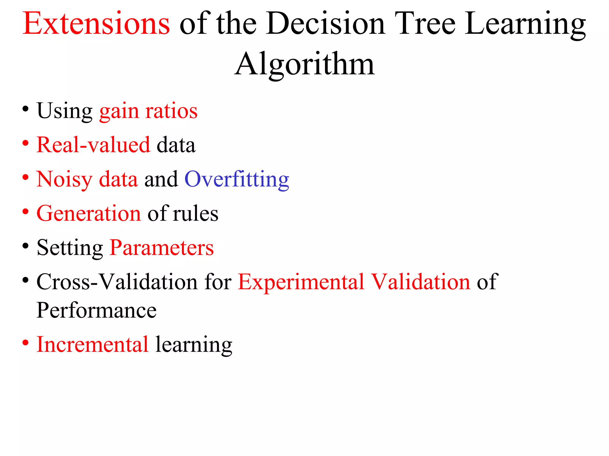
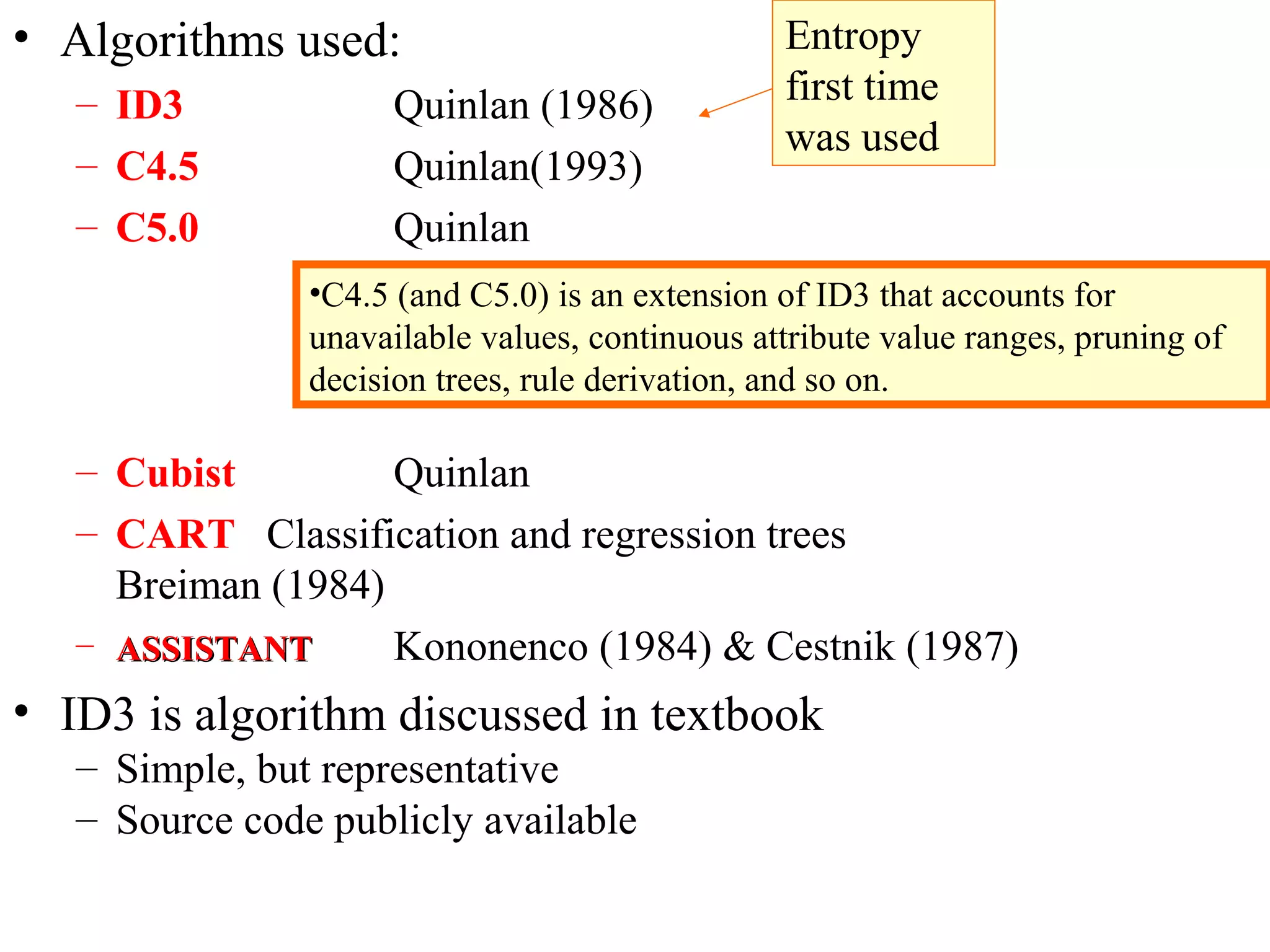
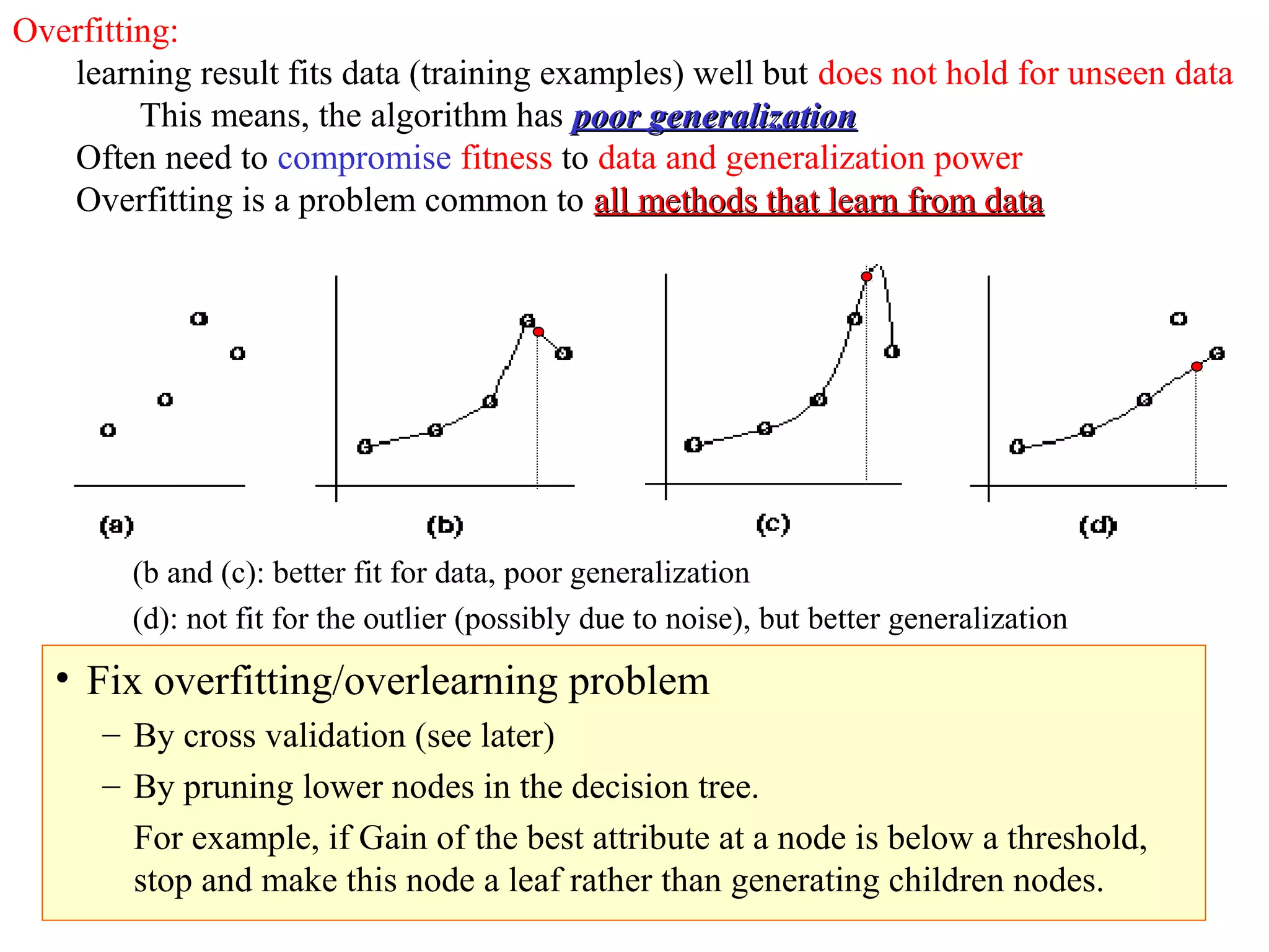
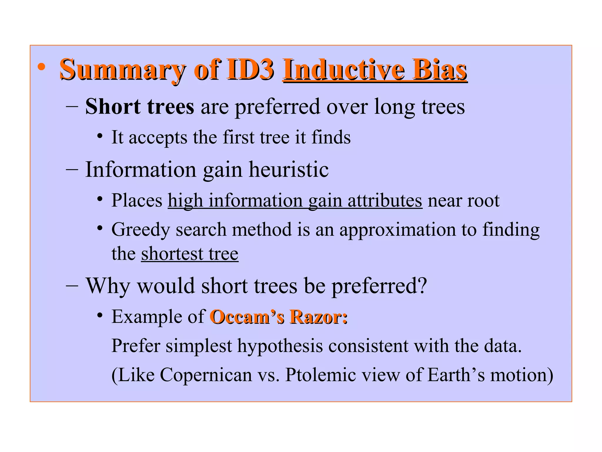
The document discusses decision tree learning, which is a machine learning approach for classification that builds classification models in the form of a decision tree. It describes the ID3 algorithm, which is a popular method for generating a decision tree from a set of training data. The ID3 algorithm uses information gain as the splitting criterion to recursively split the training data into purer subsets based on the values of the attributes. It selects the attribute with the highest information gain to make decisions at each node in the tree. Entropy from information theory is used to measure the information gain, with the goal being to build a tree that best classifies the training instances into target classes. An example applying the ID3 algorithm to a tennis playing dataset is provided to illustrate

1. Machine
Learning
Approach bbaasseedd oonn DDeecciissiioonn TTrreeeess

2. • DDeecciissiioonn TTrreeee LLeeaarrnniinngg
– Practical inductive inference method
– Same goal as Candidate-Elimination algorithm
• Find Boolean function of attributes
• Decision trees can be extended to functions with
more than two output values.
–Widely used
– Robust to noise
– Can handle disjunctive (OR’s) expressions
– Completely expressive hypothesis space
– Easily interpretable (tree structure, if-then rules)

3. TTrraaiinniinngg EExxaammpplleess
Attribute, variable,
Object, sample, property
example
SShhaallll wwee ppllaayy tteennnniiss ttooddaayy?? ((TTeennnniiss 11))
decision

4. Shall we play tennis
today?
• DDeecciissiioonn ttrreeeess ddoo
ccllaassssiiffiiccaattiioonn
– Classifies instances
into one of a discrete
set of possible
categories
– Learned function
represented by tree
– Each node in tree is
test on some attribute
of an instance
– Branches represent
values of attributes
– Follow the tree from
root to leaves to find
the output value.

5. • The tree itself forms hypothesis
– Disjunction (OR’s) of conjunctions (AND’s)
– Each path from root to leaf forms conjunction
of constraints on attributes
– Separate branches are disjunctions
• Example from PlayTennis decision tree:
(Outlook=Sunny ÙHumidity=Normal)
Ú
(Outlook=Overcast)
Ú
(Outlook=Rain Ù Wind=Weak)

6. • TTyyppeess ooff pprroobblleemmss ddeecciissiioonn ttrreeee lleeaarrnniinngg
iiss ggoooodd ffoorr::
– Instances represented by attribute-value pairs
• For algorithm in book, attributes take on a small
number of discrete values
• Can be extended to real-valued attributes
– (numerical data)
• Target function has discrete output values
• Algorithm in book assumes Boolean functions
• Can be extended to multiple output values

7. – Hypothesis space can include disjunctive expressions.
• In fact, hypothesis space is complete space of finite discrete-valued
functions
– Robust to imperfect training data
• classification errors
• errors in attribute values
• missing attribute values
• Examples:
– Equipment diagnosis
– Medical diagnosis
– Credit card risk analysis
– Robot movement
– Pattern Recognition
• face recognition
• hexapod walking gates

8. • ID3 Algorithm
– Top-down, greedy search through space of
possible decision trees
• Remember, decision trees represent hypotheses,
so this is a search through hypothesis space.
–What is top-down?
• How to start tree?
– What attribute should represent the root?
• As you proceed down tree, choose attribute for
each successive node.
• No backtracking:
– So, algorithm proceeds from top to bottom

9. The ID3 algorithm is used to build a decision tree, given a set of non-categorical attributes
C1, C2, .., Cn, the categorical attribute C, and a training set T of records.
function ID3 (R: a set of non-categorical attributes,
C: the categorical attribute,
S: a training set) returns a decision tree;
begin
If S is empty, return a single node with value Failure;
If every example in S has the same value for categorical
attribute, return single node with that value;
If R is empty, then return a single node with most
frequent of the values of the categorical attribute found in
examples S; [note: there will be errors, i.e., improperly
classified records];
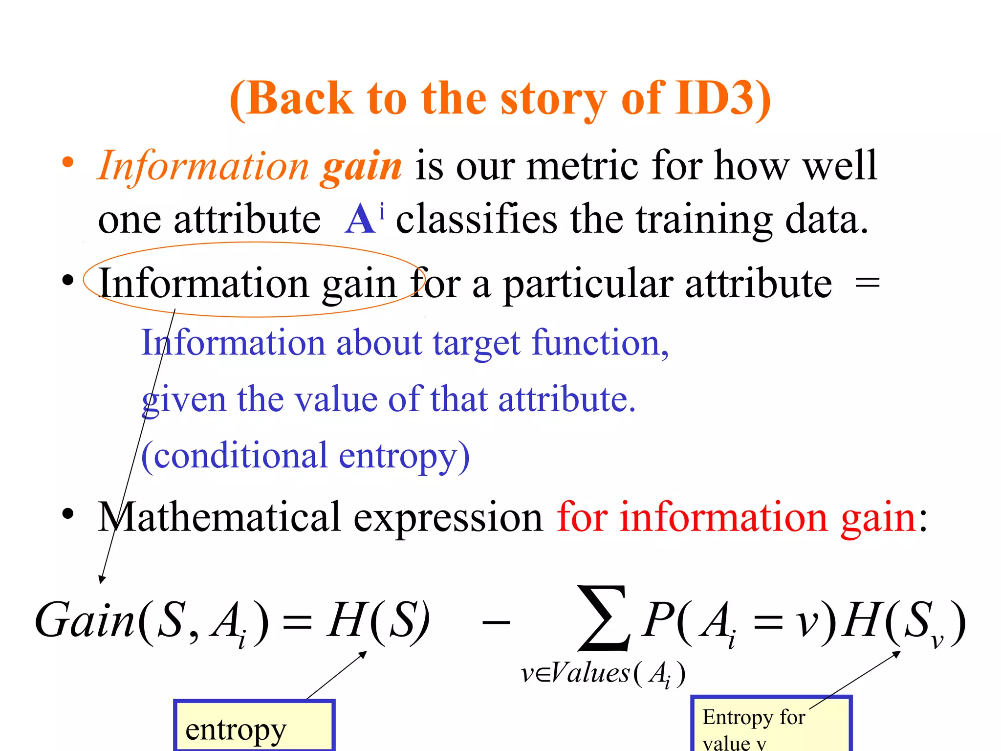
Let D be attribute with largest Gain(D,S) among R’s attributes;
Let {dj| j=1,2, .., m} be the values of attribute D;
Let {Sj| j=1,2, .., m} be the subsets of S consisting
respectively of records with value dj for attribute D;
Return a tree with root labeled D and arcs labeled
d1, d2, .., dm going respectively to the trees
ID3(R-{D},C,S1), ID3(R-{D},C,S2) ,.., ID3(R-{D},C,Sm);
end ID3;

10. –What is a greedy search?
• At each step, make decision which makes greatest
improvement in whatever you are trying optimize.
• Do not backtrack (unless you hit a dead end)
• This type of search is likely not to be a globally
optimum solution, but generally works well.
–What are we really doing here?
• At each node of tree, make decision on which
attribute best classifies training data at that point.
• Never backtrack (in ID3)
• Do this for each branch of tree.
• End result will be tree structure representing a
hypothesis which works best for the training data.

11. Information Theory Background
• If there are n equally probable possible messages, then the
probability p of each is 1/n
• Information conveyed by a message is -log(p) = log(n)
• Eg, if there are 16 messages, then log(16) = 4 and we need 4
bits to identify/send each message.
• In general, if we are given a probability distribution
P = (p1, p2, .., pn)
• the information conveyed by distribution (aka Entropy of P) is:
I(P) = -(p1*log(p1) + p2*log(p2) + .. + pn*log(pn))

12. Question?
How do you determine which
attribute best classifies data?
Answer: Entropy!
• Information gain:
– Statistical quantity measuring how well an
attribute classifies the data.
• Calculate the information gain for each attribute.
• Choose attribute with greatest information gain.

13. • But how do you measure information?
– Claude Shannon in 1948 at Bell Labs established the
field of information theory.
– Mathematical function, Entropy, measures information
content of random process:
• Takes on largest value when events are
equiprobable.
• Takes on smallest value when only one event has
non-zero probability.
– For two states:
• Positive examples and Negative examples from set S:
H(S) = -p+log2(p+) - p-log2(p-)
Entropy of set S denoted by HH((SS))

14. Entropy
Largest
entropy
Boolean
functions
with the same
number of
ones and
zeros have
largest
entropy

15. • But how do you measure information?
– Claude Shannon in 1948 at Bell Labs established the
field of information theory.
– Mathematical function, Entropy, measures information
content of random process:
• Takes on largest value when events are
equiprobable.
• Takes on smallest value when only one event has
non-zero probability.
– For two states:
• Positive examples and Negative examples from set S:
H(S) = - p+log2(p+) - p- log2(p-)
Entropy = Measure of order in set S

16. • In general:
– For an ensemble of random events: {A1,A2,...,An},
occurring with probabilities: z ={P(A1),P(A2),...,P(An)}
H P A P A i i
= å
i
n
=-
( ) log ( ( )) 2
1
n
i å £ £
(Note: = 1 and 0 1 )
1
P(A ) P(A ) i
i=
If you consider the self-information of event, i, to be: -log2(P(Ai))
Entropy is wweeiigghhtteedd aavveerraaggee of information carried by each event.
DDooeess tthhiiss mmaakkee sseennssee??

17. – If an event conveys information, that means it’s
a surprise.
– If an event always occurs, P(Ai)=1, then it
carries no information. -log2(1) = 0
– If an event rarely occurs (e.g. P(Ai)=0.001), it
carries a lot of info. -log2(0.001) = 9.97
– The less likely the event, the more the
information it carries since, for 0 £ P(Ai) £ 1,
-log2(P(Ai)) increases as P(Ai) goes from 1 to 0.
• (Note: ignore events with P(Ai)=0 since they never
occur.)
–DDooeess tthhiiss mmaakkee sseennssee??

18. • What about entropy?
– Is it a good measure of the information carried by an
ensemble of events?
– If the events are equally probable, the entropy is
maximum.
11)) For N events, each occurring with probability 1/N.
H = -å(1/N)log2(1/N) = -log2(1/N)
This is the maximum value.
(e.g. For N=256 (ascii characters) -log2(1/256) = 8
number of bits needed for characters.
Base 2 logs measure information in bits.)
This is a good thing since an ensemble of equally
probable events is as uncertain as it gets.
(Remember, information corresponds to surprise - uncertainty.)

19. –2) H is a continuous function of the probabilities.
• That is always a good thing.
–33)) If you sub-group events into compound events,
the entropy calculated for these compound
groups is the same.
• That is good since the uncertainty is the same.
• IItt iiss aa rreemmaarrkkaabbllee ffaacctt tthhaatt tthhee eeqquuaattiioonn ffoorr
eennttrrooppyy sshhoowwnn aabboovvee ((uupp ttoo aa mmuullttiipplliiccaattiivvee
ccoonnssttaanntt)) iiss tthhee oonnllyy ffuunnccttiioonn wwhhiicchh ssaattiissffiieess
tthheessee tthhrreeee ccoonnddiittiioonnss..

20. • Choice of base 2 log corresponds to
choosing units of information.(BIT’s)
• AAnnootthheerr rreemmaarrkkaabbllee tthhiinngg::
–This is the same definition of entropy used in
statistical mechanics for the measure of
disorder.
– Corresponds to macroscopic thermodynamic
quantity of Second Law of Thermodynamics.

21. • The concept of a quantitative measure for information
content plays an important role in many areas:
• For example,
– Data communications (channel capacity)
– Data compression (limits on error-free encoding)
• Entropy in a message corresponds to minimum number
of bits needed to encode that message.
• In our case, for a set of training data, the entropy
measures the number of bits needed to encode
classification for an instance.
– Use probabilities found from entire set of training data.
– Prob(Class=Pos) = Num. of positive cases / Total case
– Prob(Class=Neg) = Num. of negative cases / Total cases

22. (Back to the story of ID3)
• Information gain is our metric for how well
one attribute A i classifies the training data.
• Information gain for a particular attribute =
Information about target function,
given the value of that attribute.
(conditional entropy)
• Mathematical expression for information gain:
Gain S A = H S) - P A =
v H S i i v
( , ) ( ( ) ( )
v Values Ai
( )
Î
å
entropy Entropy for
value v

23. • ID3 algorithm (for boolean-valued function)
– Calculate the entropy for all training examples
• positive and negative cases
• p+ = #pos/Tot p- = #neg/Tot
• H(S) = -p+log2(p+) - p-log2(p-)
– Determine which single attribute best classifies the
training examples using information gain.
• For each attribute find:
å
Gain S A = H S) - P A =
v H S i i v
( , ) ( ( ) ( )
v Values Ai
( )
Î
• Use attribute with greatest information gain aass aa rroooott

24. Using Gain Ratios
• The notion of Gain introduced earlier favors attributes that have a
large number of values.
– If we have an attribute D that has a distinct value for each
record, then Info(D,T) is 0, thus Gain(D,T) is maximal.
• To compensate for this Quinlan suggests using the following ratio
instead of Gain:
GainRatio(D,T) = Gain(D,T) / SplitInfo(D,T)
• SplitInfo(D,T) is the information due to the split of T on the basis
of value of categorical attribute D.
SplitInfo(D,T) = I(|T1|/|T|, |T2|/|T|, .., |Tm|/|T|)
where {T1, T2, .. Tm} is the partition of T induced by value of D.

25. • Example: PlayTennis
– Four attributes used for classification:
• Outlook = {Sunny,Overcast,Rain}
• Temperature = {Hot, Mild, Cool}
• Humidity = {High, Normal}
• Wind = {Weak, Strong}
– One predicted (target) attribute (binary)
• PlayTennis = {Yes,No}
– Given 14 Training examples
• 9 positive
• 5 negative

26. TTrraaiinniinngg EExxaammpplleess Examples,
minterms,
cases, objects,
test cases,

27. 14 cases 9 positive cases
• Step 1: Calculate entropy for all cases:
NPos = 9 NNeg = 5 NTot = 14
H(S) = -(9/14)*log2(9/14) - (5/14)*log2(5/14) = 0.940
entropy

28. • Step 2: Loop over all attributes, calculate
gain:
– Attribute = Outlook
• Loop over values of Outlook
Outlook = Sunny
NPos = 2 NNeg = 3 NTot = 5
H(Sunny) = -(2/5)*log2(2/5) - (3/5)*log2(3/5) = 0.971
Outlook = Overcast
NPos = 4 NNeg = 0 NTot = 4
H(Sunny) = -(4/4)*log24/4) - (0/4)*log2(0/4) = 0.00

29. Outlook = Rain
NPos = 3 NNeg = 2 NTot = 5
H(Sunny) = -(3/5)*log2(3/5) - (2/5)*log2(2/5) = 0.971
• Calculate Information Gain for attribute Outlook
Gain(S,Outlook) = H(S) - NSunny/NTot*H(Sunny)
- NOver/NTot*H(Overcast)
- NRain/NTot*H(Rainy)
Gain(S,Outlook) = 9.40 - (5/14)*0.971 - (4/14)*0 - (5/14)*0.971
Gain(S,Outlook) = 0.246
– Attribute = Temperature
• (Repeat process looping over {Hot, Mild, Cool})
Gain(S,Temperature) = 0.029

30. – Attribute = Humidity
• (Repeat process looping over {High, Normal})
Gain(S,Humidity) = 0.029
– Attribute = Wind
• (Repeat process looping over {Weak, Strong})
Gain(S,Wind) = 0.048
Find attribute wwiitthh ggrreeaatteesstt iinnffoorrmmaattiioonn
ggaaiinn::
Gain(S,Outlook) = 0.246, Gain(S,Temperature) = 0.029
Gain(S,Humidity) = 0.029, Gain(S,Wind) = 0.048
Outlook is root node of tree

31. – Iterate algorithm to find attributes which
best classify training examples under the
values of the root node
– Example continued
• Take three subsets:
– Outlook = Sunny (NTot = 5)
– Outlook = Overcast (NTot = 4)
–Outlook = Rainy (NTot = 5)
• For each subset, repeat the above calculation
looping over all attributes other than Outlook

32. – For example:
• Outlook = Sunny (NPos = 2, NNeg=3, NTot = 5) H=0.971
– Temp = Hot (NPos = 0, NNeg=2, NTot = 2) H = 0.0
– Temp = Mild (NPos = 1, NNeg=1, NTot = 2) H = 1.0
– Temp = Cool (NPos = 1, NNeg=0, NTot = 1) H = 0.0
Gain(SSunny,Temperature) = 0.971 - (2/5)*0 - (2/5)*1 - (1/5)*0
Gain(SSunny,Temperature) = 0.571
Similarly:
Gain(SSunny,Humidity) = 0.971
Gain(SSunny,Wind) = 0.020
Humidity classifies Outlook=Sunny
instances best and is placed as the node under
Sunny outcome.
– Repeat this process for Outlook = Overcast &Rainy

33. –Important:
• Attributes are excluded from consideration
if they appear higher in the tree
– Process continues for each new leaf node
until:
• Every attribute has already been included
along path through the tree
or
• Training examples associated with this leaf
all have same target attribute value.

34. – End up with tree:

35. – Note: In this example data were perfect.
• No contradictions
• Branches led to unambiguous Yes, No decisions
• If there are contradictions take the majority vote
– This handles noisy data.
– Another note:
• Attributes are eliminated when they are assigned to
a node and never reconsidered.
– e.g. You would not go back and reconsider Outlook
under Humidity
– ID3 uses all of the training data at once
• Contrast to Candidate-Elimination
• Can hhaannddllee nnooiissyy ddaattaa..

36. Another Example: Russell’s and Norvig’s
Restaurant Domain
• Develop a decision tree to model the decision a patron
makes when deciding whether or not to wait for a table at
a restaurant.
• Two classes: wait, leave
• Ten attributes: alternative restaurant available?, bar in
restaurant?, is it Friday?, are we hungry?, how full is the
restaurant?, how expensive?, is it raining?,do we have a
reservation?, what type of restaurant is it?, what's the
purported waiting time?
• Training set of 12 examples
• ~ 7000 possible cases

37. A Training Set

38. A decision Tree
from Introspection

39. ID3 Induced
Decision Tree

40. ID3
• A greedy algorithm for Decision Tree Construction developed by
Ross Quinlan, 1987
• Consider a smaller tree a better tree
• Top-down construction of the decision tree by recursively
selecting the "best attribute" to use at the current node in the tree,
based on the examples belonging to this node.
– Once the attribute is selected for the current node, generate
children nodes, one for each possible value of the selected
attribute.
– Partition the examples of this node using the possible values of
this attribute, and assign these subsets of the examples to the
appropriate child node.
– Repeat for each child node until all examples associated with a
node are either all positive or all negative.

41. Choosing the Best Attribute
• The key problem is choosing which attribute to split a
given set of examples.
• Some possibilities are:
– Random: Select any attribute at random
– Least-Values: Choose the attribute with the smallest number
of possible values (fewer branches)
– Most-Values: Choose the attribute with the largest number of
possible values (smaller subsets)
– Max-Gain: Choose the attribute that has the largest expected
information gain, i.e. select attribute that will result in the
smallest expected size of the subtrees rooted at its children.
• The ID3 algorithm uses the Max-Gain method of selecting
the best attribute.

42. Splitting
Examples
by Testing
Attributes

43. Another example: Tennis 2
(simplified former example)

44. Choosing the first split

45. Resulting Decision Tree

46. • The entropy is the average number of
bits/message needed to represent a stream of
messages.
• Examples:
–if P is (0.5, 0.5) then I(P) is 1
–if P is (0.67, 0.33) then I(P) is 0.92,
–if P is (1, 0) then I(P) is 0.
• The more uniform is the probability
distribution, the greater is its information
gain/entropy.

47. • What is the hypothesis space for decision tree
learning?
– Search through space of all possible decision trees
• from simple to more complex guided by a heuristic:
information gain
– The space searched is complete space of finite,
discrete-valued functions.
• Includes disjunctive and conjunctive expressions
– Method only maintains one current hypothesis
• In contrast to Candidate-Elimination
– Not necessarily global optimum
• attributes eliminated when assigned to a node
• No backtracking
• Different trees are possible

48. • Inductive Bias: (restriction vs. preference)
– ID3
• searches complete hypothesis space
• But, incomplete search through this space looking for
simplest tree
• This is called a preference (or search) bias
– Candidate-Elimination
• Searches an incomplete hypothesis space
• But, does a complete search finding all valid hypotheses
• This is called a restriction (or language) bias
– Typically, preference bias is better since you do
not limit your search up-front by restricting
hypothesis space considered.

49. How well does it work?
Many case studies have shown that decision trees are aatt
lleeaasstt aass aaccccuurraattee aass hhuummaann eexxppeerrttss..
–A study for diagnosing breast cancer:
• humans correctly classifying the examples 65% of the time,
• the decision tree classified 72% correct.
–British Petroleum designed a decision tree for gas-oil
separation for offshore oil platforms/
• It replaced an earlier rule-based expert system.
–Cessna designed an airplane flight controller using
90,000 examples and 20 attributes per example.

50. Extensions of the Decision Tree Learning
Algorithm
• Using gain ratios
• Real-valued data
• Noisy data and Overfitting
• Generation of rules
• Setting Parameters
• Cross-Validation for Experimental Validation of
Performance
• Incremental learning

51. • Algorithms used:
– ID3 Quinlan (1986)
– C4.5 Quinlan(1993)
– C5.0 Quinlan
– Cubist Quinlan
– CART Classification and regression trees
Breiman (1984)
– AASSSSIISSTTAANNTT Kononenco (1984) & Cestnik (1987)
• ID3 is algorithm discussed in textbook
– Simple, but representative
– Source code publicly available
Entropy
first time
was used
•C4.5 (and C5.0) is an extension of ID3 that accounts for
unavailable values, continuous attribute value ranges, pruning of
decision trees, rule derivation, and so on.

52. Real-valued data
• Select a set of thresholds defining intervals;
– each interval becomes a discrete value of the attribute
• We can use some simple heuristics
– always divide into quartiles
• We can use domain knowledge
– divide age into infant (0-2), toddler (3 - 5), and school aged
(5-8)
• or treat this as another learning problem
– try a range of ways to discretize the continuous variable
– Find out which yield “better results” with respect to some
metric.

53. Noisy data and Overfitting
• Many kinds of "noise" that could occur in the examples:
– Two examples have same attribute/value pairs, but different classifications
– Some values of attributes are incorrect because of:
• Errors in the data acquisition process
• Errors in the preprocessing phase
– The classification is wrong (e.g., + instead of -) because of some error
• Some attributes are irrelevant to the decision-making process,
– e.g., color of a die is irrelevant to its outcome.
– Irrelevant attributes can result in overfitting the training data.

54. Overfitting:
learning result fits data (training examples) well but does not hold for unseen data
This means, the algorithm has ppoooorr ggeenneerraalliizzaattiioonn
Often need to compromise fitness to data and generalization power
Overfitting is a problem common to aallll mmeetthhooddss tthhaatt lleeaarrnn ffrroomm ddaattaa
(b and (c): better fit for data, poor generalization
(d): not fit for the outlier (possibly due to noise), but better generalization
• Fix overfitting/overlearning problem
– By cross validation (see later)
– By pruning lower nodes in the decision tree.
For example, if Gain of the best attribute at a node is below a threshold,
stop and make this node a leaf rather than generating children nodes.

55. Pruning Decision Trees
• Pruning of the decision tree is done by replacing a whole subtree
by a leaf node.
• The replacement takes place if a decision rule establishes that the
expected error rate in the subtree is greater than in the single leaf.
E.g.,
– Training: eg, one training red success and one training blue Failures
– Test: three red failures and one blue success
– Consider replacing this subtree by a single Failure node.
• After replacement we will have only two errors instead of five
failures.
Color
red blue
1 success
0 failure
0 success
1 failure
Color
FAILURE
red blue 2 success
1 success
3 failure
1 success
1 failure
4 failure

56. Incremental Learning
• Incremental learning
– Change can be made with each training example
– Non-incremental learning is also called batch learning
– Good for
• adaptive system (learning while experiencing)
• when environment undergoes changes
– Often with
• Higher computational cost
• Lower quality of learning results
– ITI (by U. Mass): incremental DT learning package

57. Evaluation Methodology
• Standard methodology: cross validation
1. Collect a large set of examples (all with correct classifications!).
2. Randomly divide collection into two disjoint sets: training and
test.
3. Apply learning algorithm to training set giving hypothesis H
4. Measure performance of H w.r.t. test set
• Important: keep the training and test sets disjoint!
• Learning is not to minimize training error (wrt data) but
the error for test/cross-validation: a way to fix overfitting
• To study the efficiency and robustness of an algorithm,
repeat steps 2-4 for different training sets and sizes of
training sets.
• If you improve your algorithm, start again with step 1 to
avoid evolving the algorithm to work well on just this
collection.

58. Restaurant Example
Learning Curve

59. Decision Trees to Rules
• It is easy to derive a rule set from a decision tree: write a rule for
each path in the decision tree from the root to a leaf.
• In that rule the left-hand side is easily built from the label of the
nodes and the labels of the arcs.
• The resulting rules set can be simplified:
– Let LHS be the left hand side of a rule.
– Let LHS' be obtained from LHS by eliminating some conditions.
– We can certainly replace LHS by LHS' in this rule if the subsets of the
training set that satisfy respectively LHS and LHS' are equal.
– A rule may be eliminated by using metaconditions such as "if no other rule
applies".

60. C4.5
• C4.5 is an extension of ID3 that accounts for
unavailable values, continuous attribute value
ranges, pruning of decision trees, rule derivation,
and so on.
C4.5: Programs for Machine Learning
J. Ross Quinlan, The Morgan Kaufmann Series
in Machine Learning, Pat Langley,
Series Editor. 1993. 302 pages.
paperback book & 3.5" Sun
disk. $77.95. ISBN 1-55860-240-2

61. Summary of DT Learning
• Inducing decision trees is one of the most widely used learning
methods in practice
• Can out-perform human experts in many problems
• Strengths include
– Fast
– simple to implement
– can convert result to a set of easily interpretable rules
– empirically valid in many commercial products
– handles noisy data
• Weaknesses include:
– "Univariate" splits/partitioning using only one attribute at a time so limits
types of possible trees
– large decision trees may be hard to understand
– requires fixed-length feature vectors

62. • SSuummmmaarryy ooff IIDD33 IInndduuccttiivvee BBiiaass
– Short trees are preferred over long trees
• It accepts the first tree it finds
– Information gain heuristic
• Places high information gain attributes near root
• Greedy search method is an approximation to finding
the shortest tree
– Why would short trees be preferred?
• Example of OOccccaamm’’ss RRaazzoorr::
Prefer simplest hypothesis consistent with the data.
(Like Copernican vs. Ptolemic view of Earth’s motion)

63. – Homework Assignment
• Tom Mitchell’s software
See:
• http://www.cs.cmu.edu/afs/cs.cmu.edu/project/theo-3/www/ml.html
• Assignment #2 (on decision trees)
• Software is at: http://www.cs.cmu.edu/afs/cs/project/theo-3/mlc/hw2/
– Compiles with gcc compiler
– Unfortunately, README is not there, but it’s easy to figure out:
» After compiling, to run:
dt [-s <random seed> ] <train %> <prune %> <test %> <SSV-format data file>
» %train, %prune, & %test are percent of data to be used for training, pruning &
testing. These are given as decimal fractions. To train on all data, use 1.0 0.0 0.0
– Data sets for PlayTennis and Vote are include with code.
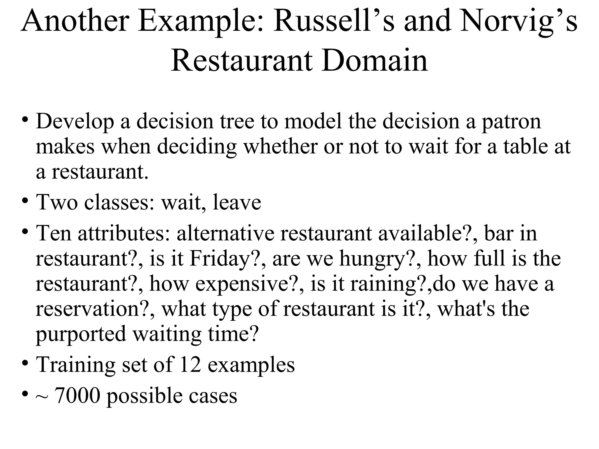
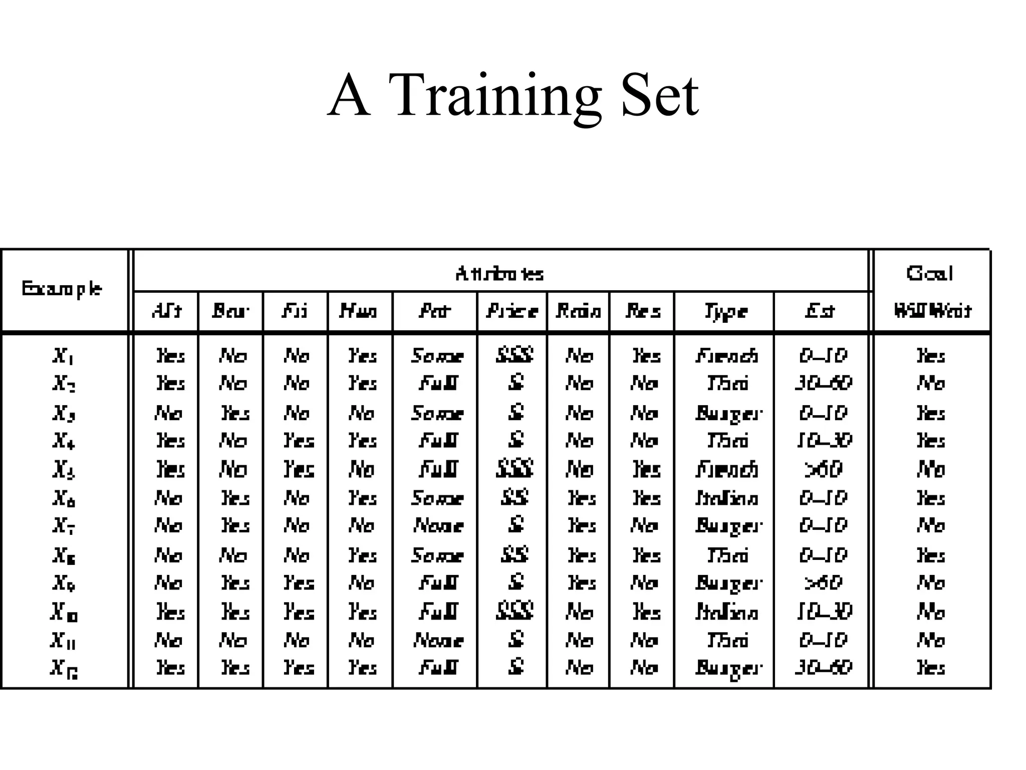
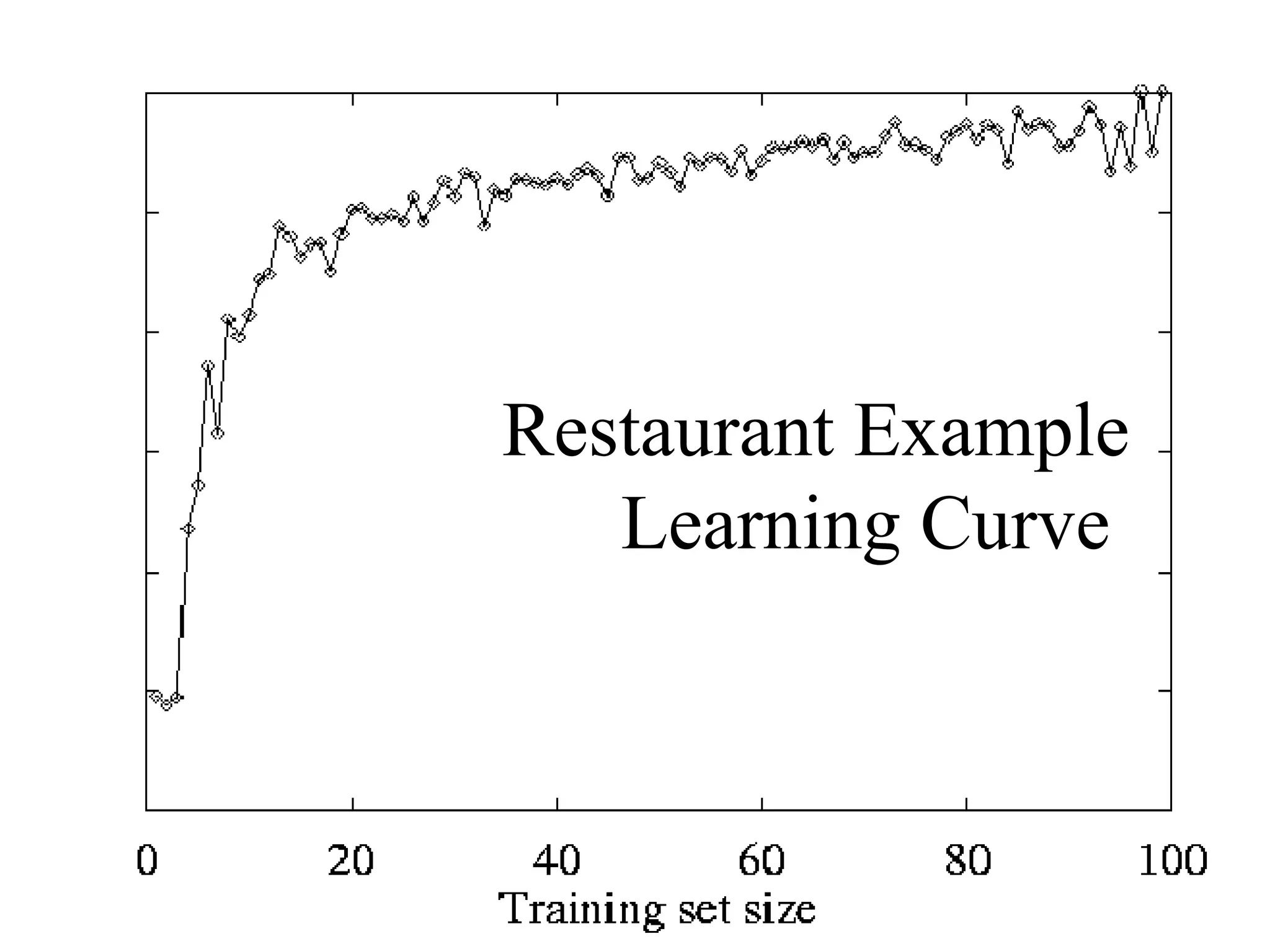
– Also try the Restaurant example from Russell & Norvig
– Also look at www.kdnuggets.com/ (Data Sets)
Machine Learning Database Repository at UC Irvine - (try “zoo” for fun)

64. QQuueessttiioonnss aanndd PPrroobblleemmss
• 1. Think how the method of finding best variable
order for decision trees that we discussed here be
adopted for:
• ordering variables in binary and multi-valued decision
diagrams
• finding the bound set of variables for Ashenhurst and other
functional decompositions
• 2. Find a more precise method for variable ordering in
trees, that takes into account special function patterns
recognized in data
• 3. Write a Lisp program for creating decision trees with
entropy based variable selection.

65. – Sources
• Tom Mitchell
– Machine Learning, Mc Graw Hill 1997
• Allan Moser
• Tim Finin,
• Marie desJardins
• Chuck Dyer