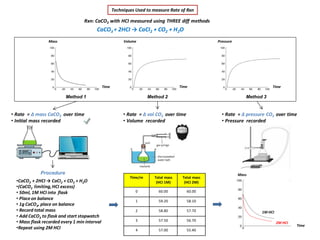
The document describes techniques used to measure the rate of reactions. Three different methods are used to measure the rate of reaction between calcium carbonate and hydrochloric acid: 1) change in mass of calcium carbonate over time, 2) volume of carbon dioxide produced over time, and 3) change in pressure of carbon dioxide over time. Data from each method using 1M and 2M hydrochloric acid is shown in a table. Two additional reactions are described which use two methods each: change in absorbance over time and change in a visual property (disappearance of a cross or change in mass) over time.

1. Techniques Used to measure Rate of Rxn
Rxn: CaCO3 with HCI measured using THREE diff methods
CaCO3 + 2HCI → CaCI2 + CO2 + H2O
• Rate = Δ mass CaCO3 over time
• Initial mass recorded
•CaCO3 + 2HCI → CaCI2 + CO2 + H2O
•(CaCO3 limiting,HCI excess)
• 50ml, 1M HCI into flask
• Place on balance
• 1g CaCO3, place on balance
• Record total mass
• Add CaCO3 to flask and start stopwatch
• Mass flask recorded every 1 min interval
•Repeat using 2M HCI
Method 1 Method 3Method 2
Mass
Time Time Time
Volume Pressure
• Rate = Δ vol CO2 over time
• Volume recorded
• Rate = Δ pressure CO2 over time
• Pressure recorded
Procedure
Time/m Total mass
(HCI 1M)
Total mass
(HCI 2M)
0 60.00 60.00
1 59.20 58.10
2 58.80 57.70
3 57.50 56.70
4 57.00 55.40
Mass
Time
2M HCI
1M HCI

2. Techniques Used to measure Rate of Rxn
Rxn: CaCO3 with HCI measured using THREE diff methods
CaCO3 + 2HCI → CaCI2 + CO2 + H2O
• Rate = Δ mass CaCO3 over time
• Initial mass recorded
•CaCO3 + 2HCI → CaCI2 + CO2 + H2O
•(CaCO3 limiting,HCI excess)
• 50ml, 1M HCI into flask
• Add 1g CaCO3 to flask and start stopwatch
• Vol recordedevery 1 min interval
•Repeat using 2M HCI
Method 1 Method 3Method 2
Mass
Time Time Time
Volume Pressure
• Rate = Δ vol CO2 over time
• Volume recorded
• Rate = Δ pressure CO2 over time
• Pressure recorded
Procedure
Time/m Vol CO2
(HCI 1M)
Vol CO2
(HCI 2M)
0 0.0 0.0
1 8.5 14.0
2 15.0 26.5
3 21.0 34.0
4 26.0 39.0
Volume CO2
Time
2M HCI
1M HCI

3. Techniques Used to measure Rate of Rxn
Rxn: CaCO3 with HCI measured using THREE diff methods
CaCO3 + 2HCI → CaCI2 + CO2 + H2O
• Rate = Δ mass CaCO3 over time
• Initial mass recorded
•CaCO3 + 2HCI → CaCI2 + CO2 + H2O
•(CaCO3 limiting,HCI excess)
• 50ml, 1M HCI into flask
• Add 1gCaCO3 to flask and start stopwatch
• Press recorded every 1 min interval
•Repeat using 2M HCI
Method 1 Method 3Method 2
Mass
Time Time Time
Volume Pressure
• Rate = Δ vol CO2 over time
• Volume recorded
• Rate = Δ pressure CO2 over time
• Pressure recorded
Procedure
Time/m Pressure CO2
(HCI 1M)
Pressure CO2
(HCI 2M)
0 101.3 101.3
1 102.4 103.4
2 103.5 105.6
3 110.3 115.2
4 113.5 118.2
Pressure CO2
Time
2M HCI
1M HCI

4. Techniques Used to measure Rate of Rxn
• Rate = Δ mass Sulfur over time
Method 1 Method 2
Mass
Time Time
Light Intensity
• Rate = Δ light intensity over time
• Light intensity recorded
Procedure Conc/M
S2O3
2-
Time/s Rate
1/Time
0.2 80.8 1/80.8 = 0.0123
0.4 40.2 1/40.2 = 0.0248
0.6 25.2 1/25.2 = 0.0396
0.8 20.5 1/20.5 = 0.0487
1.0 18.2 1/18.2 = 0.0550
Rate = 1/time
Conc
Rxn: Na2S2O3 with HCI measured using TWO diff methods
Na2S2O3 + 2HCI → 2NaCI2 + SO2 + H2O + S
• Na2S2O3 + 2HCI → 2NaCI2 + SO2 + H2O + S
• (Na2S2O3 limiting, HCI excess)
•50ml 0.2M HCI into conical flask
• Place on top of paper with cross X
• Pour 5ml 0.1M Na2S2O3 into flask
• Record time for X to disappear
• Repeat with diff S2O3
2-
conc
Light sensor
Light source
0.2 0.4 0.6 0.8

5. • Na2S2O3 + 2HCI → 2NaCI2 + SO2 + H2O + S
• (Na2S2O3 limiting, HCI excess)
•Pipette 1ml 0.2M S2O3
2-
into cuvette
• Pipette 0.1ml 0.1M HCI into cuvette
• Mix and start light sensor
• Record time for light intensity to drop
• Repeat with diff S2O3
2-
conc
Techniques Used to measure Rate of Rxn
• Rate = Δ mass Sulfur over time
Method 1 Method 2
Mass
Time Time
Light Intensity
• Rate = Δ light intensity over time
• Light intensity recorded
Procedure Conc/M
S2O3
2-
Time/s Rate
1/Time
0.2 80.8 1/80.8 = 0.0123
0.4 40.2 1/40.2 = 0.0248
0.6 25.2 1/25.2 = 0.0396
0.8 20.5 1/20.5 = 0.0487
1.0 18.2 1/18.2 = 0.0550
Rate = 1/time
Rxn: Na2S2O3 with HCI measured using TWO diff methods
Na2S2O3 + 2HCI → 2NaCI2 + SO2 + H2O + S
Light source
Light sensor
Light intensity
0.8M
S2O3
2-
1M
S2O3
2-
Conc
0.2 0.4 0.6 0.818.2 20.3 time

6. • H2O2 + 2KI + 2HCI → 2KCI + 2H2O + I2
(KIlimiting, H2O2 excess)
• Pipette 5ml 3% H2O2, 5ml 0.1M HCI into flask
• Add starch, 1ml 0.1M S2O3 to flask
• Place on white paper with cross X
• Pipette 5 ml 0.1M KI into flask
• Record time for X to disappear
• Repeat with diff KI conc
Techniques Used to measure Rate of Rxn
Method 1 Method 2
Mass iodine produced
Time Time
Absorbance
• Rate = Δ Absorbance over time
• Absorbance recorded
Procedure Conc/M
KI
Time/s Rate
1/Time
0.00625 80.8 1/80.8 = 0.0123
0.0125 40.2 1/40.2 = 0.0248
0.025 25.2 1/25.2 = 0.0396
0.05 20.5 1/20.5 = 0.0487
0.1 18.2 1/18.2 = 0.0550
Rate = 1/time
Conc
Rxn: H2O2 with I -
measured using TWO diff methods
H2O2 + 2I- + 2H+ → 2H2O + I2
Iodine Clock Rxn
H2O2 + 2I - + 2H+ → 2H2O + I2
I2 + 2S2O3
2-
→ S4O6
2-
+ 2I -
I2 + starch → Blue black
H2O2 - Oxidising Agent
I - - Reducing Agent
S203
2-
- Reduce I2 to I –
I2 - I2 react with starch
form blue black
• Rate = Δ mass iodine over time
= Disappearance X due to blue black formation
Abs increase when
blue black form
0.025 0.05 0.1

7. • H2O2 + 2KI + 2HCI → 2KCI + 2H2O + I2
(KIlimiting, H2O2 excess)
• Pipette 0.5ml 3% H2O2, 0.1M HCI to cuvette
• Add starch, 0.1ml 0.1M S2O3 to cuvette
• Pipette 0.5ml 0.2M KI to cuvette
• Record Abs change
• Repeat with diff KI conc
Techniques Used to measure Rate of Rxn
Method 1 Method 2
Mass iodine produced
Time Time
Absorbance
• Rate = Δ Absorbance over time
• Absorbance recorded
Procedure Absorbance
Time
Abs increase when
blue black form
Rxn: H2O2 with I -
measured using TWO diff methods
H2O2 + 2I- + 2H+ → 2H2O + I2
Iodine Clock Rxn
H2O2 + 2I - + 2H+ → 2H2O + I2
I2 + 2S2O3
2-
→ S4O6
2-
+ 2I -
I2 + starch → Blue black
H2O2 - Oxidising Agent
I - - Reducing Agent
S203
2-
- Reduce I2 to I –
I2 - I2 react with starch
form blue black
• Rate = Δ mass iodine over time
= Disappearance X due to blue black formation
Time Conc KI
(0.2)
Abs
Conc KI
(0.4)
Abs
Conc KI
(0.6)
Abs
Conc KI
(0.8)
Abs
0 0.1 0.1 0.1 0.1
2 0.1 0.1 0.1 0.1
4 0.1 0.1 0.1 1.4
6 0.1 0.1 1.2
8 0.1 0.1
10 0.1 1.3
12 0.1
Rate 1/14
= 0.07
1/10
= 0.1
1/6
= 0.16
1/ 4
= 0.25
000000.2M KI0.8M KI
4 6 10 12

8. Techniques Used to measure Rate of Rxn
Method 1 Method 2
Mass iodine produced
Time Time
Absorbance
• Rate = Δ Absorbance over time
• Absorbance recorded
Procedure Conc KI
/M
Time/s Rate
1/Time
0.00625 80.8 1/80.8 = 0.0123
0.0125 40.2 1/40.2 = 0.0248
0.025 25.2 1/25.2 = 0.0396
0.05 20.5 1/20.5 = 0.0487
0.1 18.2 1/18.2 = 0.0550
Rate = 1/time
Conc
Rxn: S2O8
2-
with I -
measured using TWO diff methods
Iodine Clock Rxn
S2O8
2
- Oxidising Agent
I - - Reducing Agent
S203
2-
- Reduce I2 to I –
I2 - I2 react with starch
form blue black
• Rate = Δ mass iodine over time
= Disappearance X due to blue black formation
Abs increase when
blue black form
S2O8
2-
+ 2I -
→ 2SO4
2-
+ I2
S2O8
2-
+ 2I - → 2SO4
2-
+ I2
I2 + 2 S203
2-
→ S406
2-
+ 2I -
I2 + starch → Blue black
• S2O8
2-
+ 2I -
→ 2SO4
2-
+ I2
(KIlimiting, S2O8
2-
excess)
• Pipette 5ml 0.1M KI, 0.1M S2O3
• Add 1ml starch to flask
• Place on white paper with cross X
• Pipette 5 ml 0.1M S2O8
2-
to flask
• Record time for X to disappear
• Repeat with diff KI conc
0.0125 0.025 0.05 0.1

9. • S2O8
2-
+ 2I -
→ 2SO4
2-
+ I2
(KIlimiting, S2O8
2-
excess)
• Pipette 0.5ml 0.1M KI, 0.1M S2O3 to cuvette
• Add 0.1ml starch to cuvette
• Pipette 0.5ml 0.1M S2O8
2-
to cuvette
• Record Abs change
• Repeat with diff KI conc
Techniques Used to measure Rate of Rxn
Method 1 Method 2
Mass iodine produced
Time Time
Absorbance
• Rate = Δ Absorbance over time
• Absorbance recorded
Procedure
Rxn: S2O8
2-
with I -
measured using TWO diff methods
Iodine Clock Rxn
S2O8
2
- Oxidising Agent
I - - Reducing Agent
S203
2-
- Reduce I2 to I –
I2 - I2 react with starch
form blue black
• Rate = Δ mass iodine over time
= Disappearance X due to blue black formation
Abs increase when
blue black form
S2O8
2-
+ 2I -
→ 2SO4
2-
+ I2
S2O8
2-
+ 2I - → 2SO4
2-
+ I2
I2 + 2 S203
2-
→ S406
2-
+ 2I -
I2 + starch → Blue black
Time Conc KI
(0.2)
Abs
Conc KI
(0.4)
Abs
Conc KI
(0.6)
Abs
Conc KI
(0.8)
Abs
0 0.1 0.1 0.1 0.1
2 0.1 0.1 0.1 0.1
4 0.1 0.1 0.1 1.4
6 0.1 0.1 1.2
8 0.1 0.1
10 0.1 1.3
12 0.1
Rate 1/14
= 0.07
1/10
= 0.1
1/6
= 0.16
1/ 4
= 0.25
Absorbance
Time
0.8M KI
00000000000.2M KI
4 6 10 12

10. Techniques Used to measure Rate of Rxn
Method 1 Method 2
Time Time
Volume Pressure
• Rate = Δ vol O2 over time
• Volume recorded
• Rate = Δ pressure O2 over time
• Pressure recorded
Procedure
2H2O2 → O2 + 2H2O
Rxn: H2O2 with KI (catalyst)measured using TWO diff methods
• 2H2O2 → O2 + 2H2O
(H2O2 limiting,KI excess)
• Pipette 1ml 1.0M KI to 20ml of 1.5% H2O2
• Vol O2 released recordedat 1 min interval
• Repeated using 3% H2O2 conc
Time/m Vol O2
(H2O2 1.5%)
Vol O2
(H2O2 3.0%)
0 0.0 0.0
1 8.5 14.0
2 15.0 26.5
3 21.0 34.0
4 26.0 39.0
Volume O2
Time
3 %
1.5 %

11. • 2H2O2 → O2 + 2H2O
(H2O2 limiting,KI excess)
• Pipette 1ml 1.0M KI to 20ml of 1.5% H2O2
• Pressure O2 released recorded at 1 min interval
• Repeat using 3% H2O2 conc
Techniques Used to measure Rate of Rxn
Method 1 Method 2
Time Time
Volume Pressure
• Rate = Δ vol O2 over time
• Volume recorded
• Rate = Δ pressure O2 over time
• Pressure recorded
Procedure
2H2O2 → O2 + 2H2O
Time
3 %
1.5 %
Time/m Pressure O2
(H2O2 1.5%)
Pressure O2
(H2O2 3%)
0 101.3 101.3
1 102.4 103.4
2 103.5 105.6
3 110.3 115.2
4 113.5 118.2
Pressure O2
Rxn: H2O2 with KI (catalyst)measured using TWO diff methods

12. • Rate = Δ Conc I2 over time
• Conc recorded using titration
Techniques Used to measure Rate of Rxn
Method 1 Method 2
Conc iodine produced
Time Time
Absorbance
• Rate = Δ Absorbance over time
• Absorbance recorded
Procedure
Absorbance
Time
Abs increase when
iodine form
2Fe3+
+ 2I -
→ 2Fe2+
+ I2
Rxn: Fe3+
+ I -
measured using TWO diff methods
Fe 3+
- Oxidising Agent
I - - ReducingAgent
• 2Fe3+
+ 2I -
→ 2Fe2+
+ I2
•(I -
limiting, Fe3+
excess)
• Pipette 1.5ml 0.02M Fe3+
to cuvette.
• Find λ max for Fe3+
(450nm)
• Abs vs time , select λ = 450nm
• Pipette 1.0ml 0.02M KI to cuvette
• Measure abs increase due to I2 formation
• Repeat using diff KI conc
Time/s Conc 0.02M KI
Abs
Conc 0.04M KI
Abs
0 0.240 0.240
1 0.245 0.260
2 0.257 0.330
3 0.300 0.390
4 0.330 0.540
0.04 M
0.02 M

13. • 2Fe3+
+ 2I -
→ 2Fe2+
+ I2
(I -
limiting, Fe3+
excess)
• Pipette 25ml 0.02M KI /Fe3+
to flask.
• Start time
• Every 5min, pipette 10ml sol mix to flask
• Titrate with S2O3
2-
( I2 form will react with S2O3
2-
)
Amt I2 produced is determine.
• I2 + 2S203
2-
→ S4O6
2-
+ 2I –
(Mol ratio 1:2)
• Rate = Δ Conc I2 over time
• Conc recorded using titration
Techniques Used to measure Rate of Rxn
Method 1 Method 2
Conc iodine produced
Time Time
Absorbance
• Rate = Δ Absorbance over time
• Absorbance recorded
Procedure
Conc I2
Time
2Fe3+
+ 2I -
→ 2Fe2+
+ I2
Rxn: Fe3+
+ I -
measured using TWO diff methods
Fe 3+
- Oxidising Agent
I - - ReducingAgent
Time/m Vol S2O3/ cm3 Conc I2/M
0 0 0
5 6 0.06
10 18 0.18
15 28 0.28
20 28 0.28
25 ml 0.02M
KI/Fe3+
10ml removed
every 5m
0.2M S2O3
3-
Contain I2
2S203
2-
+ I2 → S4O6
2-
+ 2I –
2 mol S203
2
– 1 mol I2
0.0012 mol – 0.006 mol I2
Vol S203
2-
6.0ml – Amt S203
2-
= M x V
= 0.2 x 0.006
= 0.0012 mol
Conc I2 = Amt I2/Vol
= 0.0006/0.01
= 0.06 M

14. • I2 + CH3COCH3 → CH3COCH2I + H+
+ I –
(CH3COCH3 limiting, I2 excess)
• Pipette 1ml 0.002M I2 to cuvette.
• Abs vs Time (λ max = 520nm)
• Pipette 0.4ml 2M HCI and 1ml water to cuvette
• Pipette 0.4ml 0.2M CH3COCH3 to cuvette
• Record drop in abs over time
• Repeat using diff CH3COCH3 conc
• Rate = Δ Conc I2 over time
• Conc recorded
Techniques Used to measure Rate of Rxn
Method 1 Method 2
Conc iodine
Time Time
Absorbance I2
• Rate = Δ Absorbance over time
• Absorbance recorded
Procedure
Time
Abs decrease
I2 consumed
I2 + CH3COCH3 → CH3COCH2I + H+
+ I -
Rxn: I2 + CH3COCH3 measured using TWO diff methods
Time Conc
(0.2M)
Abs
Conc
(0.4M)
Abs
Conc
(0.6M)
Abs
0 2.00 2.00 2.00
2 1.86 1.76 1.52
4 1.75 1.54 1.20
6 1.57 1.24 0.78
8 1.23 1.23 0.56
10 1.10 0.78 0.40
Rate Gradient
Time 0
Gradient
Time 0
Gradient
Time 0
Absorbance I2
0.2 M
0.4 M0.6 M
Conc CH3COCH3
Rate

15. • Rate = Δ Conc I2 over time
• Conc obtain from std calibrationplot
Techniques Used to measure Rate of Rxn
Method 1 Method 2
Conc iodine
Time Time
Absorbance I2
• Rate = Δ Absorbance over time
• Absorbance recorded
Procedure
I2 + CH3COCH3 → CH3COCH2I + H+
+ I -
Rxn: I2 + CH3COCH3 measured using TWO diff methods
Time Conc I2
(0.2M)
Abs
Conc I2
(0.4M)
Abs
Conc I2
(0.6M)
Abs
0 2.00 2.00 2.00
2 1.86 1.76 1.52
4 1.75 1.54 1.20
6 1.57 1.24 0.78
Absorbance I2
0.2 M
0.4 M0.6 M
Conc I2
• I2 + CH3COCH3 → CH3COCH2I + H+
+ I –
(CH3COCH3 limiting, I2 excess)
• Pipette 1ml 0.002M I2 to cuvette.
• Prepare std calibration plot Abs vs I2 conc
• Abs vs Time (λ max = 520nm)
• Pipette 0.4ml 2M HCI and 1ml water to cuvette
• Pipette 0.4ml 0.2M CH3COCH3 to cuvette
• Record drop in abs over time
• Repeat using diff I2 conc
Convert Abs I2 to conc I2
using std calibration curve
Time
0.2 M
0.4 M0.6 M
Conc I2 Abs
0 0
0.125 0.3
0.25 0.5
0.5 0.7
1.0 1.1
Std calibration curve
Time

16. GraphicalRepresentationof Order :ZERO, FIRST and SECOND order
ZERO ORDER FIRST ORDER SECOND ORDER
Rate – 2nd order respect to [A]
Conc x2 – Rate x 4
Unit for k
Rate = k[A]2
Rate = kA2
k = M-1s-1
Rate
Conc reactant
Rate
Conc reactant Conc reactant
Conc Conc Conc
Time Time Time
Time
Conc reactant
Rate
Time
ln At
Time
1/At
ktAA ot  ][][
Rate = k[A]0
Rate independent of [A]
Unit for k
Rate = k[A]0
Rate = k
k = Ms-1
Rate vs Conc – Constant
Conc vs Time – Linear
Rate = k[A]1
Rate - 1st order respect to [A]
Unit for k
Rate = k[A]1
Rate = kA
k = s-1
Rate vs Conc - proportional
Conc vs Time
ktAA
eAA
ot
kt
ot

 
]ln[]ln[
][][
[A]t
[A]o
kt
AA ot

][
1
][
1
ln Ao
1/Ao
Conc at time t Conc at time t

17. Using 2nd methodto find order
Determinationorder: Na2S2O3 + 2HCI → NaCI + H2O + S + SO2
Order of Na2S2O3
Conc Na2S2O3 changes, fix [HCI] = 0.1M
Na2S2O3 added
HCI was added
Time taken X fade away
Conc
Na2S2O3
Time/s
Trial 1
±0.01
Time/s
Trial 2
±0.01
Time/s
Trial 3
±0.01
Average
time
Rate
0.05 102.96 103.23 114.80 107.00 0.00046
0.10 45.43 44.08 38.35 42.62 0.0023
0.15 27.36 27.13 26.36 26.95 0.0055
0.20 18.06 18.57 17.53 18.05 0.0111
0.25 15.26 15.44 16.88 15.86 0.0158
Result expt
00046.0
107
05.0
.

timeAve
Conc
Rate
Cal for Conc 0.05M
4 ways for uncertainty rate
1st method
Ave time = (107.00 ± 0.01)
% uncertainty time = 9.34 x 10-3 %
%∆ Rate = %∆ Time
Rate = 0.00046 ± 9.34 x 10-3 %
= 0.00046 ± 0.000000043
Too small
Poor choice
4th method
Uncertainty rate = (Max – min) for rate
Rate 1 = Conc/time 1 = 0.05 / 102.96 = 0.00049
Rate 2 = Conc/time 2 = 0.05 / 103.23 = 0.00048
Rate 3 = Conc/ time 3 = 0.05 / 114.80 = 0.00043
Max rate = 0.00049
Min rate = 0.00043
Range = (Max – Min)/2
Range = (0.00049 – 0.00043)/2
= 0.00003
Average rate = (R1 + R2 + R3)/3
= 0.00047 ± 0.00003
Consistent
Good choice
3rd method
Uncertainty rate = std deviation (for conc 0.05)
Rate 1 = Conc/time 1 = 0.05 / 102.96 = 0.00049
Rate 2 = Conc/time 2 = 0.05 / 103.23 = 0.00048
Rate 3 = Conc / time 3 = 0.05 / 114.80 = 0.00043
Average rate = (R1 + R2 + R3)/3
= 0.00047 ± std dev
= 0.00047 ± 0.000032
Consistent
Good choice
2nd method
Using Range (Max – Min) for time
Range = (Max – Min) for time/2
Range = (114.80 – 102.96)/2 = 5.92
Ave time = (107.00 ± 5.92)
% uncertainty time = 5.5%
% ∆Rate = %∆Time
Rate = 0.00046 ± 5.5%
= 0.00046 ± 0.000026
Consistent
Good choice

18. Determinationorder : Na2S2O3 + 2HCI → NaCI + H2O + S + SO2
Order of Na2S2O3
Conc Na2S2O3 changes, fix [HCI] = 0.1M
Na2S2O3 added
HCI was added
Time taken X fade away
Conc
Na2S2O3
Time/s
Trial 1
±0.01
Time/s
Trial 2
±0.01
Time/s
Trial 3
±0.01
Average
time
Rate
0.05 102.96 103.23 114.80 107.00 0.00046
0.10 45.43 44.08 38.35 42.62 0.0023
0.15 27.36 27.13 26.36 26.95 0.0055
0.20 18.06 18.57 17.53 18.05 0.0111
0.25 15.26 15.44 16.88 15.86 0.0158
Result expt
00046.0
00.107
05.0
.

timeAve
Conc
Rate
Cal for Conc 0.05M
2nd method
Using Range (Max – Min) for time
Range = (Max – Min)/2
Range = (114.80 – 102.96)/2 = 5.92
Ave time = (107.00 ± 5.92)
% uncertainty time = 5.5%
% ∆Rate = %∆Time
Rate = 0.00046 ± 5.5%
= 0.00046 ± 0.000026
Consistent
Good choice
Uncertaintyrate for conc 0.05M
Conc
Na2S2O3
Time/s
Trial 1
±0.01
Time/s
Trial 2
±0.01
Time/s
Trial 3
±0.01
Average
time
± Time
Range (Max- Min)/2
% ±Time Rate(±rate)
0.05 102.96 103.23 114.80 107.00 (114.8-102.96)/2= 5.92 5.5% 0.00046±0.000026
0.10 45.43 44.08 38.35 42.62 (45.43 – 38.35)/2 = 3.54 8.3% 0.0023 ±0.00027
0.15 27.36 27.13 26.36 26.95 (27.13 – 26.36)/2 = 0.50 1.8% 0.0055 ±0.00022
0.20 18.06 18.57 17.53 18.05 (18.06 – 17.53)/2 = 0.52 2.8% 0.0111 ±0.0006
0.25 15.26 15.44 16.88 15.86 (16.88 – 15.26)/2 = 0.81 5.1% 0.0158 ±0.0011

19. Determinationorder: Na2S2O3 + 2HCI → NaCI + H2O + S + SO2
Plot of Conc vs Rate
Conc
Na2S2O3
Rate(±rate)
0.05 0.00046±0.0000026
0.10 0.0023 ±0.00027
0.15 0.0055 ±0.00022
0.20 0.0111 ±0.0006
0.25 0.0158 ±0.0011
Order for Na2S2O3 (fix conc HCI)
Let Rate = k[Na2S2O3]x [HCI] y
Rate
Conc Na2S2O3
Uncertainty rate
Conc Na2S2O3
Rate
Best fit
Order = 2.21
Best fit
Order = 2.21
Max fit
Order = 2.29
Min fit
Order = 2.12
Lowest uncertainty (Lowest Conc)
to
Highest uncertainty (Highest Conc)
Highest uncertainty (Lowest Conc)
to
Lowest uncertainty (Highest Conc)
Max order
Min order

20. Determinationorder: Na2S2O3 + 2HCI → NaCI + H2O + S + SO2
Conc
Na2S2O3
Rate(±rate)
0.05 0.00046±0.0000026
0.10 0.0023 ±0.00027
0.15 0.0055 ±0.00022
0.20 0.0111 ±0.0006
0.25 0.0158 ±0.0011
Conc
Na2S2O3
Rate(±rate)
0.05 0.00044
0.10 0.00221
0.15 0.0055
0.20 0.0114
0.25 0.017
Max order
Max fit
Order = 2.29
Max order – Lowest uncertainty (Lowest Conc) to Highest uncertainty (Highest Conc)
Conc
Na2S2O3
Rate(±rate)
0.05 0.00046±0.0000026
0.10 0.0023 ±0.00027
0.15 0.0055 ±0.00022
0.20 0.0111 ±0.0006
0.25 0.0158 ±0.0011
Min order
Conc
Na2S2O3
Rate(±rate)
0.05 0.00048
0.10 0.00248
0.15 0.0055
0.20 0.0108
0.25 0.0147
Conc Na2S2O3
Conc Na2S2O3
Rate
Rate
Min fit
Order = 2.12
Min order – Highest uncertainty (Lowest Conc) to Lowest uncertainty (Highest Conc)
Highest uncertainty
0.0158 + 0.0011
= 0.017
Lowest uncertainty
0.00046 – 0.000026
= 0.00044
Highest uncertainty
0.00046 + 0.000026
= 0.00048
Lowest uncertainty
0.0158 – 0.0011
= 0.0147
Lowest uncertainty
Highest uncertainty
Lowest uncertainty
Highest uncertainty
Max order
Min order

21. Order respect to Na2S2O3 = 2.21
Theoretical order = 2.00
% Error order = 10.7%
Determinationorder: Na2S2O3 + 2HCI → NaCI + H2O + S + SO2
Conc
Na2S2O3
Rate(±rate)
0.05 0.00046±0.0000026
0.10 0.0023 ±0.00027
0.15 0.0055 ±0.00022
0.20 0.0111 ±0.0006
0.25 0.0158 ±0.0011
Order for Na2S2O3 (fix conc HCI)
Let Rate = k[Na2S2O3]x [HCI] 1
Order x = 2.21
Conc Na2S2O3
Rate
Best fit
Order = 2.21
Max fit
Order = 2.29
Min fit
Order = 2.12
Uncertainty order = (Max order – Min order)/2
%7.10%100
00.2
)00.221.2(


± Uncertaintyfor order = (Max – Min order)/2
Max order = 2.29
Min order = 2.12
± Uncertaintyorder
(Max – Min)/2 = ( 2.29 – 2.12)/2
= 0.09
± Uncertaintyorder = 2.21 ± 0.09
% uncertainty order = (0.09/2.21)x 100 %
= 4%
% Error order = 10.7%
% Uncertainty
(Random Error)
% Uncertainty
(SystematicError)
4%
% Error = % Random + % Systematic
error error
% Systematic = (10.7 – 4 )= 6.7%
error
Correct Method !

22. Order respect to Na2S2O3 = 2.21
Theoretical order = 2.00
% Error order = 10.7%
Determinationorder: Na2S2O3 + 2HCI → NaCI + H2O + S + SO2
Conc
Na2S2O3
Rate(±rate)
0.05 0.00046±0.0000026
0.10 0.0023 ±0.00027
0.15 0.0055 ±0.00022
0.20 0.0111 ±0.0006
0.25 0.0158 ±0.0011
Order for Na2S2O3 (fix conc HCI)
Let Rate = k[Na2S2O3]x [HCI] 1
Order x = 2.21
Conc Na2S2O3
Rate
Best fit
Order = 2.21
% Uncertainty rate = % Uncertainty time = 5.5%
%7.10%100
00.2
)00.221.2(


% Error order = 10.7%
% Uncertainty
(Random Error)
% Uncertainty
(SystematicError)
5.5%
Conc
Na2S2O3
Time/s
Trial 1
±0.01
Time/s
Trial 2
±0.01
Time/s
Trial 3
±0.01
Average
time
± Time
Range (Max- Min)/2
% ±Time
0.05 102.96 103.23 114.80 107.00 (114.8-102.96)/2= 5.92 5.5%
0.10 45.43 44.08 38.35 42.62 (45.43 – 38.35)/2 = 3.54 8.3%
0.15 27.36 27.13 26.36 26.95 (27.13 – 26.36)/2 = 0.50 1.8%
0.20 18.06 18.57 17.53 18.05 (18.06 – 17.53)/2 = 0.52 2.8%
0.25 15.26 15.44 16.88 15.86 (16.88 – 15.26)/2 = 0.81 5.1%
Wrong Method !
% Error = % Random + % Systematic
error error
% Systematic = (10.7 – 5.5)= 5.2 %
error