Downloaded 66 times
![IOSR Journal of Mechanical and Civil Engineering (IOSR-JMCE)
e-ISSN: 2278-1684,p-ISSN: 2320-334X, Volume 9, Issue 5 (Nov. - Dec. 2013), PP 58-64
www.iosrjournals.org
www.iosrjournals.org 58 | Page
A Simple Case Study of Material Requirement Planning
Asis Sarkar1
, Dibyendu Das2
, Sujoy Chakraborty3
, Nabarun Biswas4
1,2,3,4
Assistant Professor
1,2
Department of Mechanical Engineering, 3
Department of Production Engineering, N.I.T.Agartala, Jirania,
Barjala-799055,Tripura, India.
4
Department of Mechanical Engineering
N.I.T.M.A.S, Dimond Harbour, West Bengal, India.
Abstract: A material requirement planning is a technique that uses the bill of material, inventory data and a
master schedule to calculate requirements for material. It also takes into account the combination of the bill of
material structure and assembly lead times. The result of an MRP plan is a material plan for each item found in
the bill of material structure which indicates the amount of new material required, the date on which it is
required. The new schedule dates for material that is currently on order. If routings, with defined labor
requirements are available, a capacity plan will be created concurrently with the MRP material plan. The MRP
plan can be run for any number entities (which could be physically separated inventories) and can include
distributor inventories, if the system has access to this type of information. MRP tries to strike the best balance
possible between optimizing the service level and minimizing costs and capital lockup. In this paper it is tried
to present a practical M.R.P. problem and is shown how it is helpful in optimizing the service level and
minimizing costs.
Keywords: material requirement planning; inventory; bill of materials; master schedule; optimizing.
I. Introduction
Traditionally, manufacturing companies have controlled their parts through the reorder point (ROP)
technique. Gradually, they recognized that some of these components had dependent demand, and material
requirements planning (MRP) evolved to control the dependent items more effectively. MRP has been a very
popular and widely used multilevel inventory control method since 1970s. The application of this popular tool in
materials management has greatly reduced inventory levels and improved productivity (Wee and Shum,
1999).The introduced MRP was the first version of MRP system, named as Materials Requirements Planning
(MRP I). Later, several MRP systems were extended into other versions including Manufacturing Resources
Planning (MRP II) and Enterprise Resources Planning (ERP) (Browne et al., 1996). MRP is a commonly
accepted approach for replenishment planning in major companies. The MRP based software tools are accepted
readily. Most industrial decision makers are familiar with their use. The practical aspect of MRP lies in the fact
that this is based on comprehensible rules, and provides cognitive support, as well as a powerful information
system for decision
Materials requirements planning (MRP) is an inventory planning and control technique developed to
deal with dependent-demand inventories. An MRP system, in its simplest form, consists of three basic
components: a master production schedule (MPS); bill-of-material (BOM) files of the end items; and inventory
status files of various materials, components, parts, subassemblies and final products [I]. The MPS is a product
requirements schedule compiled from both firm customer orders and tentative demand forecasts. It is a listing of
the demand for the end items in each of the time periods over a planning horizon. Given the MPS, the
requirements of the lower-level components and parts can be derived using the information contained in the
various BOM files. These lower-level material requirements are then backward scheduled into the appropriate
time periods according to the planned lead times specified in the BOM. These time-phased gross material
requirements are modified by the amount of materials on hand and on order for each time period by consulting
the inventory status files. The net requirements of each material in each time period can then be computed.
Finally, orders are placed for materials with positive net requirements. An important decision problem in MRP
is determining the size of production lots from the net requirements. A production lot is a batch of parts
continuously produced under the same operating conditions. The problem of determining the quantities of parts
to be processed in a batch and the times of completing these batches is commonly referred to as the lot-sizing
problem in the literature.
One of its main objectives is to keep the due date equal to the need date, eliminating material shortages
and excess stocks. MRP breaks a component into parts and subassemblies, and plans for those parts to come into
stock when needed. Material requirement planning systems help manufactures determine precisely when and
how much material to purchase and process based upon a time phased analysis of sales orders, production](https://image.slidesharecdn.com/i0955864-150120222747-conversion-gate01/85/A-Simple-Case-Study-of-Material-Requirement-Planning-1-320.jpg)
![IOSR Journal of Mechanical and Civil Engineering (IOSR-JMCE)
e-ISSN: 2278-1684,p-ISSN: 2320-334X, Volume 9, Issue 5 (Nov. - Dec. 2013), PP 58-64
www.iosrjournals.org
www.iosrjournals.org 58 | Page
A Simple Case Study of Material Requirement Planning
Asis Sarkar1
, Dibyendu Das2
, Sujoy Chakraborty3
, Nabarun Biswas4
1,2,3,4
Assistant Professor
1,2
Department of Mechanical Engineering, 3
Department of Production Engineering, N.I.T.Agartala, Jirania,
Barjala-799055,Tripura, India.
4
Department of Mechanical Engineering
N.I.T.M.A.S, Dimond Harbour, West Bengal, India.
Abstract: A material requirement planning is a technique that uses the bill of material, inventory data and a
master schedule to calculate requirements for material. It also takes into account the combination of the bill of
material structure and assembly lead times. The result of an MRP plan is a material plan for each item found in
the bill of material structure which indicates the amount of new material required, the date on which it is
required. The new schedule dates for material that is currently on order. If routings, with defined labor
requirements are available, a capacity plan will be created concurrently with the MRP material plan. The MRP
plan can be run for any number entities (which could be physically separated inventories) and can include
distributor inventories, if the system has access to this type of information. MRP tries to strike the best balance
possible between optimizing the service level and minimizing costs and capital lockup. In this paper it is tried
to present a practical M.R.P. problem and is shown how it is helpful in optimizing the service level and
minimizing costs.
Keywords: material requirement planning; inventory; bill of materials; master schedule; optimizing.
I. Introduction
Traditionally, manufacturing companies have controlled their parts through the reorder point (ROP)
technique. Gradually, they recognized that some of these components had dependent demand, and material
requirements planning (MRP) evolved to control the dependent items more effectively. MRP has been a very
popular and widely used multilevel inventory control method since 1970s. The application of this popular tool in
materials management has greatly reduced inventory levels and improved productivity (Wee and Shum,
1999).The introduced MRP was the first version of MRP system, named as Materials Requirements Planning
(MRP I). Later, several MRP systems were extended into other versions including Manufacturing Resources
Planning (MRP II) and Enterprise Resources Planning (ERP) (Browne et al., 1996). MRP is a commonly
accepted approach for replenishment planning in major companies. The MRP based software tools are accepted
readily. Most industrial decision makers are familiar with their use. The practical aspect of MRP lies in the fact
that this is based on comprehensible rules, and provides cognitive support, as well as a powerful information
system for decision
Materials requirements planning (MRP) is an inventory planning and control technique developed to
deal with dependent-demand inventories. An MRP system, in its simplest form, consists of three basic
components: a master production schedule (MPS); bill-of-material (BOM) files of the end items; and inventory
status files of various materials, components, parts, subassemblies and final products [I]. The MPS is a product
requirements schedule compiled from both firm customer orders and tentative demand forecasts. It is a listing of
the demand for the end items in each of the time periods over a planning horizon. Given the MPS, the
requirements of the lower-level components and parts can be derived using the information contained in the
various BOM files. These lower-level material requirements are then backward scheduled into the appropriate
time periods according to the planned lead times specified in the BOM. These time-phased gross material
requirements are modified by the amount of materials on hand and on order for each time period by consulting
the inventory status files. The net requirements of each material in each time period can then be computed.
Finally, orders are placed for materials with positive net requirements. An important decision problem in MRP
is determining the size of production lots from the net requirements. A production lot is a batch of parts
continuously produced under the same operating conditions. The problem of determining the quantities of parts
to be processed in a batch and the times of completing these batches is commonly referred to as the lot-sizing
problem in the literature.
One of its main objectives is to keep the due date equal to the need date, eliminating material shortages
and excess stocks. MRP breaks a component into parts and subassemblies, and plans for those parts to come into
stock when needed. Material requirement planning systems help manufactures determine precisely when and
how much material to purchase and process based upon a time phased analysis of sales orders, production](https://image.slidesharecdn.com/i0955864-150120222747-conversion-gate01/75/A-Simple-Case-Study-of-Material-Requirement-Planning-1-2048.jpg)
![A Simple Case Study of Material Requirement Planning
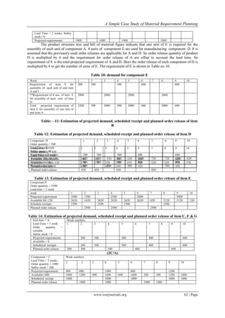
www.iosrjournals.org 64 | Page
take up the assignment on material requirement planning by correlating the production planning and inventory
management problem.
References:
[1]. J Hoey, B.R. Kilmarting and R. Leonard (1986). Designing a Material Requirement Planning System to meet the needs of low-
volume, Make – to – order companies (with case study). Int. J. Prod. Res., 24, 2, 375-386.
[2]. James R. Ashby (1995). Scheduling and Order Release in a single stage production system. J. of manufacturing systems, 14, 4,290-
306.
[3]. A.G. Lagodimos and E.J. Anderson (1993). Optimal Positioning of Safety Stocks in MRP. Int. J. Prod. Res, 31, 8, 1797-1813.
[4]. W.C. Benton and R. Srivastava (1993). Product Structure complexity and inventory storage capacity on the performance of
multilevel manufacturing system. Int. J. Prod. Res., 33, 11, 2531-2545.
[5]. Yenisey, M. M. (2006), A flownetwork approach for equilibrium of material requirements planning. International Journal of
Production Economics, 102, pp 317–332.
[6]. Mula, J., Poler, R., and Garcia, G. P. (2006), MRP with flexible constraints: a fuzzy mathematical programming approach. Fuzzy
Sets and System, 157, pp 74–97.
[7]. Wilhelm, W.E., Som, P. (1998), Analysis of a singlestage, singleproduct ,stochastic,MRPcontrolled assembly system. European
Journal of Operational Research 108, pp 74– 93
[8]. Axsäter, S. (2005), Planning order release for an assembly system with random
[9]. operations times.ORSpectrum, 27, pp 459–470.
[10]. Kanet JJ, Sridharan SV. (1998), the value of using scheduling information in planning material requirements. International Journal
of Decision Science; 29, pp 479–96.
[11]. Kumar, A. (1989), Component inventory cost in an assembly problem with uncertain supplier leadtimes.IIE Transactions 21(2), pp
112–121.
[12]. Chauhan, S.S., Dolgui, A., Proth, J.M.(2009), A continuous model for supply planning of assembly systems with stochastic
component procurement times. International Journal of Production Economics 120, pp 411–417.
[13]. Van Donselaar, K.H., Gubbels, B.J. (2002), How to release orders in order to minimize system inventory and system nervousness?
International Journal of Production Economics 78, pp 335–343.
[14]. Minifie JR, Davis RA. (1990), Interaction effects on MRP nervousness. International Journal of Production Research; 28, pp 173–
83.
[15]. Billington PJ, McClain JO, Thomas J. (1983), Mathematical programming approaches to capacity constrained MRP systems:
review, formulation and problem reduction. Management Science; 29, pp1126–41.](https://image.slidesharecdn.com/i0955864-150120222747-conversion-gate01/85/A-Simple-Case-Study-of-Material-Requirement-Planning-7-320.jpg)

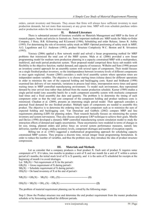
This document discusses Material Requirement Planning (MRP), a technique for managing inventory using a master schedule, bill of materials, and inventory data to optimize material requirements and minimize costs. It presents a case study involving a car assembly process to illustrate how MRP can improve service levels and efficiency in manufacturing. The methodology includes steps for determining requirements and preparing necessary orders based on production schedules and projected demands.


