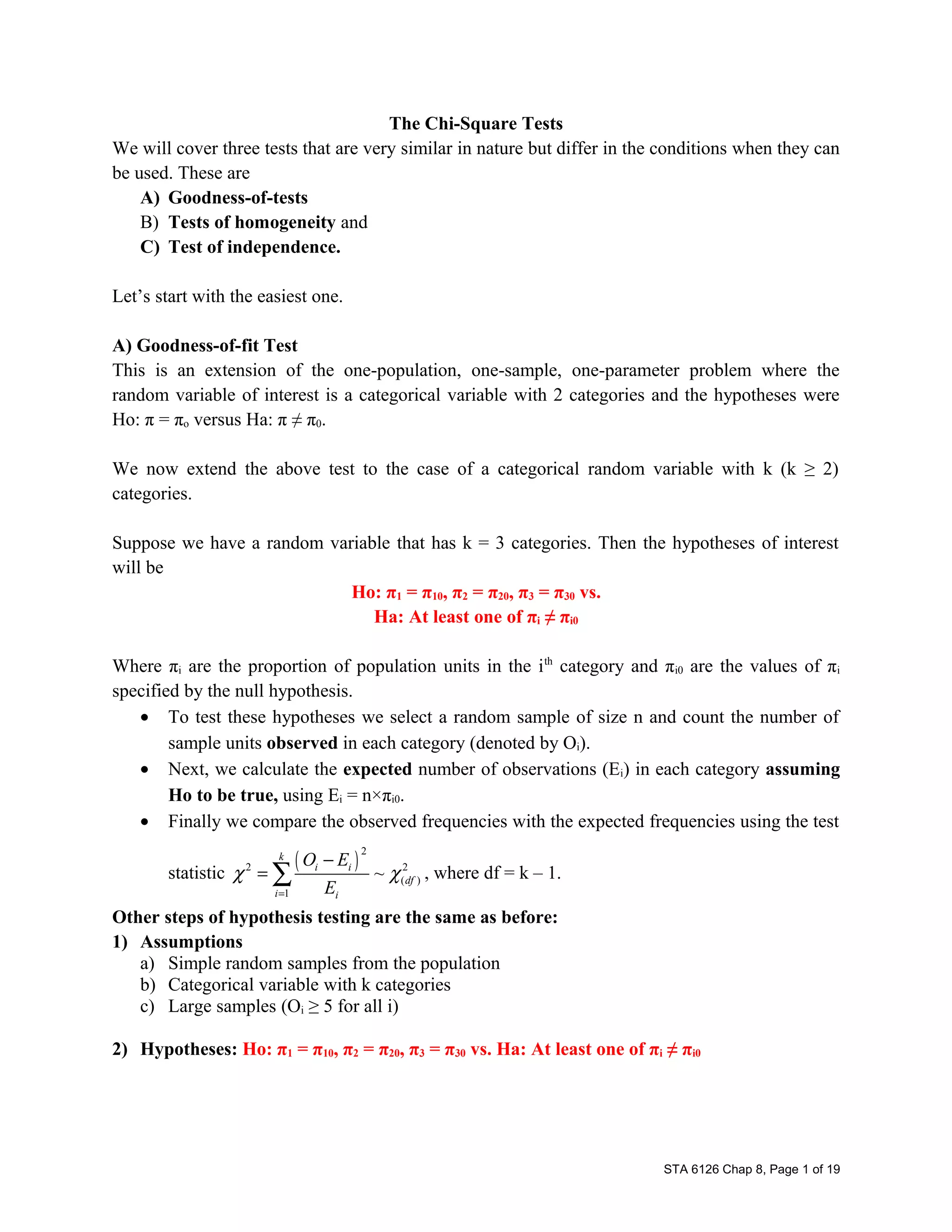
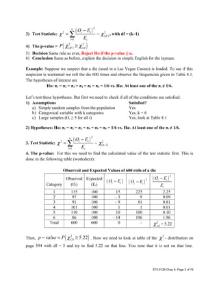
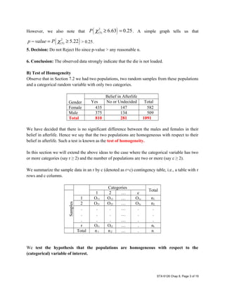
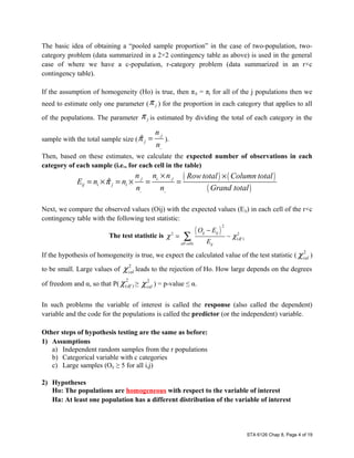
This document provides an overview of three Chi-Square tests: goodness-of-fit tests, tests of homogeneity, and tests of independence. Goodness-of-fit tests compare observed data to expected data based on a hypothesized distribution with one or more categories. Tests of homogeneity compare observed data across multiple populations to determine if they have the same distribution. Tests of independence examine the relationship between two categorical variables to determine if they are independent. All three tests use a Chi-Square test statistic and follow similar procedures: define hypotheses, calculate expected values, compare to observed values, and determine statistical significance. Examples are provided to illustrate how to set up and conduct each type of test.

1. The Chi-Square Tests
We will cover three tests that are very similar in nature but differ in the conditions when they can
be used. These are
A) Goodness-of-tests
B) Tests of homogeneity and
C) Test of independence.
Let’s start with the easiest one.
A) Goodness-of-fit Test
This is an extension of the one-population, one-sample, one-parameter problem where the
random variable of interest is a categorical variable with 2 categories and the hypotheses were
Ho: π = πo versus Ha: π ≠ π0.
We now extend the above test to the case of a categorical random variable with k (k ≥ 2)
categories.
Suppose we have a random variable that has k = 3 categories. Then the hypotheses of interest
will be
Ho: π1 = π10, π2 = π20, π3 = π30 vs.
Ha: At least one of πi ≠ πi0
Where πi are the proportion of population units in the ith
category and πi0 are the values of πi
specified by the null hypothesis.
• To test these hypotheses we select a random sample of size n and count the number of
sample units observed in each category (denoted by Oi).
• Next, we calculate the expected number of observations (Ei) in each category assuming
Ho to be true, using Ei = n×πi0.
• Finally we compare the observed frequencies with the expected frequencies using the test
statistic
( )
2
2 2
( )
1
~
k
i i
df
i i
O E
E
χ χ
=
−
= ∑ , where df = k – 1.
Other steps of hypothesis testing are the same as before:
1) Assumptions
a) Simple random samples from the population
b) Categorical variable with k categories
c) Large samples (Oi ≥ 5 for all i)
2) Hypotheses: Ho: π1 = π10, π2 = π20, π3 = π30 vs. Ha: At least one of πi ≠ πi0
STA 6126 Chap 8, Page 1 of 19

2. 3) Test Statistic:
( )
2
2 2
( )
1
~
k
i i
df
i i
O E
E
χ χ
=
−
= ∑ , with df = (k–1)
4) The p-value = ( )2 2
( )df calP χ χ≥
5) Decision Same rule as ever, Reject Ho if the p-value ≤ α.
6) Conclusion Same as before, explain the decision in simple English for the layman.
Example: Suppose we suspect that a die (used in a Las Vegas Casino) is loaded. To see if this
suspicion is warranted we roll the die 600 times and observe the frequencies given in Table 8.1.
The hypotheses of interest are
Ho: π1 = π2 = π3 = π4 = π5 = π6 = 1/6 vs. Ha: At least one of the πi ≠ 1/6.
Let’s test these hypotheses. But first we need to check if all of the conditions are satisfied:
1) Assumptions Satisfied?
a) Simple random samples from the population Yes
b) Categorical variable with k categories Yes, k = 6
c) Large samples (Oi ≥ 5 for all i) Yes, look at Table 8.1
2) Hypotheses: Ho: π1 = π2 = π3 = π4 = π5 = π6 = 1/6 vs. Ha: At least one of the πi ≠ 1/6.
3. Test Statistic:
( )
2
6
2 2
(6 1)
1
~i i
i i
O E
E
χ χ −
=
−
= ∑
4. The p-value: For this we need to find the calculated value of the test statistic first. This is
done in the following table (worksheet):
Observed and Expected Values of 600 rolls of a die
Category
Observed
(Oi)
Expected
(Ei)
( )i i
O E− ( )
2
i i
O E−
( )
2
i i
i
O E
E
−
1 115 100 15 225 2.25
2 97 100 – 3 9 0.09
3 91 100 – 9 81 0.81
4 101 100 1 1 0.01
5 110 100 10 100 0.10
6 86 100 – 14 196 1.96
Total 600 600 0 – 2
calχ = 5.22
Then, ( )2
(5) 5.22p value P χ− = ≥ . Now we need to look at table of the
2
χ - distribution on
page 594 with df = 5 and try to find 5.22 on that line. You note that it is not on that line.
STA 6126 Chap 8, Page 2 of 19

3. However, we also note that ( )2
(5) 6.63 0.25P χ ≥ = . A simple graph tells us that
( )2
(5) 5.22p value P χ− = ≥ > 0.25.
5. Decision: Do not Reject Ho since p-value > any reasonable α.
6. Conclusion: The observed data strongly indicate that the die is not loaded.
B) Test of Homogeneity
Observe that in Section 7.2 we had two populations, two random samples from these populations
and a categorical random variable with only two categories.
Gender
Belief in Afterlife
Yes No or Undecided Total
Female 435 147 582
Male 375 134 509
Total 810 281 1091
We have decided that there is no significant difference between the males and females in their
belief in afterlife. Hence we say that the two populations are homogeneous with respect to their
belief in afterlife. Such a test is known as the test of homogeneity.
In this section we will extend the above ideas to the case where the categorical variable has two
or more categories (say r ≥ 2) and the number of populations are two or more (say c ≥ 2).
We summarize the sample data in an r by c (denoted as r×c) contingency table, i.e., a table with r
rows and c columns.
Categories
Total
Samples
1 2 … c
1 O11 O12 … O1c n1.
2 O21 O22 … O2c n2.
.
.
.
.
.
.
.
.
.
…
…
…
.
.
.
.
.
.
r Or1 Or2 … . nr.
Total n.1 n.2 … . n..
We test the hypothesis that the populations are homogeneous with respect to the
(categorical) variable of interest.
STA 6126 Chap 8, Page 3 of 19

4. The basic idea of obtaining a “pooled sample proportion” in the case of two-population, two-
category problem (data summarized in a 2×2 contingency table as above) is used in the general
case of where we have a c-population, r-category problem (data summarized in an r×c
contingency table).
If the assumption of homogeneity (Ho) is true, then πij = πj for all of the j populations then we
need to estimate only one parameter ( jπ ) for the proportion in each category that applies to all
of the populations. The parameter jπ is estimated by dividing the total of each category in the
sample with the total sample size (
.
..
ˆ j
j
n
n
π = ).
Then, based on these estimates, we calculate the expected number of observations in each
category of each sample (i.e., for each cell in the table)
( ) ( )
( )
. . .
.. ..
ˆ j i j
ij i j i
n n n Row total Column total
E n n
n n Grand total
π
× ×
= × = × = =
Next, we compare the observed values (Oij) with the expected values (Eij) in each cell of the r×c
contingency table with the following test statistic:
The test statistic is
( )
2
2 2
( )~
ij ij
df
all cells ij
O E
E
χ χ
−
= ∑
If the hypothesis of homogeneity is true, we expect the calculated value of the test statistic (
2
calχ )
to be small. Large values of
2
calχ leads to the rejection of Ho. How large depends on the degrees
of freedom and α, so that P(
2
( )dfχ ≥
2
calχ ) = p-value ≤ α.
In such problems the variable of interest is called the response (also called the dependent)
variable and the code for the populations is called the predictor (or the independent) variable.
Other steps of hypothesis testing are the same as before:
1) Assumptions
a) Independent random samples from the r populations
b) Categorical variable with c categories
c) Large samples (Oij ≥ 5 for all i,j)
2) Hypotheses
Ho: The populations are homogeneous with respect to the variable of interest
Ha: At least one population has a different distribution of the variable of interest
STA 6126 Chap 8, Page 4 of 19

5. 3) Test Statistic:
( )
2
2 2
( )~
ij ij
df
all cells ij
O E
E
χ χ
−
= ∑ , with df = (r–1)(c–1),
Where,
( ) ( )
( )
. . .
.. ..
ˆ j i j
ij i j i
n n n Row total Column total
E n n
n n Grand total
π
× ×
= × = × = =
4) The p-value = ( )2 2
( )df calP χ χ≥ .
5) Decision Same rule as ever, Reject Ho if the p-value ≤ α.
6) Conclusion Same as before, explain the decision in simple English for the layman.
C) Test of Independence
This test is used in a different context but all of the steps are the same as the test of homogeneity.
We have one population and a random sample of size n (= n..). Each sample unit is asked two
questions (one of which is called the response and the other the predictor) that have r and c
categories as responses. The sample data are then summarized in an r×c contingency table as
before.
Response
Total
Predictor
1 2 … c
1 O11 O12 … O1c n1.
2 O21 O22 … O2c n2.
.
.
.
.
.
.
.
.
.
…
…
…
.
.
.
.
.
.
r Or1 Or2 … . nr.
Total n.1 n.2 … . n..
The hypotheses of interest are:
Ho: The two random variables are independent of each other.
Ha: The two random variables are associated with each other.
Everything else is the same as in the case of the test of homogeneity. Thus,
Steps in test of independence
1) Assumptions
a) Independent random samples from the r populations
b) Categorical variable with c categories
c) Large samples (Oij ≥ 5 for all i,j)
2) Hypotheses
Ho: The two random variables are independent of each other.
Ha: The two random variables are associated with each other.
STA 6126 Chap 8, Page 5 of 19

6. 3) Test Statistic:
( )
2
2 2
( )~
ij ij
df
all cells ij
O E
E
χ χ
−
= ∑ , with df = (r–1)(c–1),
Where,
( ) ( )
( )
. . .
.. ..
ˆ j i j
ij i j i
n n n Row total Column total
E n n
n n Grand total
π
× ×
= × = × = =
4) The p-value = ( )2 2
( )df calP χ χ≥
5) Decision Same rule as ever, Reject Ho if the p-value ≤ α.
6) Conclusion Same as before, explain the decision in simple English for the layman.
Let’s see how these apply to the case of 2 populations (predictor variable)and 2 samples and a
categorical variable (response) with 2 categories.
We were interested in whether or not the probability of “Success” in the two categories of the
explanatory variable are equal, that is, the hypotheses of interest were
Ho: π1 – π2 = 0 vs. Ha: π1 – π2 ≠ 0.
If Ho is true then there is only one parameter (π) and π1 = π and π2 = π.
Now let’s put these true values in a table.
Response
1 =
Success”
0 =
Failure”
Total
X=Predictor
1 π1 1- π1 1
2 π2 1- π2 1
Total π 1- π 1
Note that
π1 = Proportion of “Success”s in population 1
= P(A randomly selected item will be a “Success” when we know that the item is
selected from population 1)
= P(Y = 1 given X = 1) = P(Y = 1 | X = 1)
= Conditional probability of Y = 1 given X = 1.
Similarly we may write,
π2 = P(Y = 1 given X = 2) = Conditional probability of Y = 1 given X = 2
How about π? Well, it is the unconditional probability that Y = 1, i.e., π = P(Y = 1).
STA 6126 Chap 8, Page 6 of 19

7. When Ho is true, i.e., when the conditional probabilities are equal to the unconditional
probabilities we say “the response and the predictor are independent of each other” or that “there
is no association between the response and the predictor.”
So the test for difference of two population proportions is also a test of homogeneity of a
categorical variable. However, if we select a random sample of size n (= n..) and ask two
questions, one of which identifies the population, then we have a test of independence of two
categorical variables.
We have seen that these concepts can be extended this to the case of a categorical predictor
with 2 or more categories and a categorical response with 2 or more categories, where data
from a random sample are summarized in an r × c contingency table.
Example-1: A few years ago after the week-end when Gator Basketball team won the game that
put them in the Final Four (which ended at 11:30 p.m.), 101 students in a Statistics class were
asked to report their gender and whether or not have watched the whole game, part of it or not at
all. The following table summarizes the responses:
Watched? Gender Total
Male Female
Whole game 10 21 31
Part of Game 12 24 36
None 4 30 34
Total 26 75 101
To compare the differences in how much each gender watched the game, we need to find
percentages in each category; but first we have to decide which variable is the response and
which one is the predictor, so that we can decide what to put in the denominator of these
proportions.
In this example,
 The response is how much each student watched the game and
 The predictor is gender.
 To compare the two genders we will divide the numbers in each “cell” of the above table
by the total number of students of each gender, i.e., divide the number of observations in
each cell by the total in each predictor (gender) category
 Such a division will give how much of the game watched by gender, i.e., the conditional
distribution of response:
STA 6126 Chap 8, Page 7 of 19

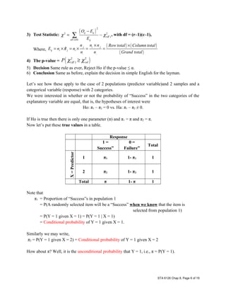
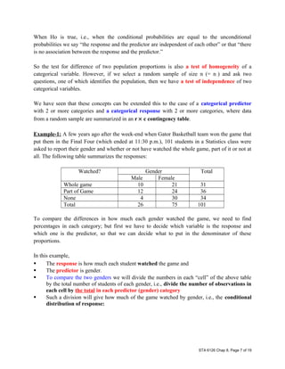
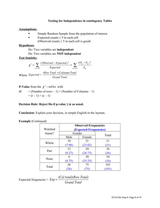
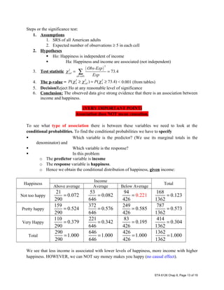
8. Conditional Distribution of Response
Watched?
Gender
Total
Male Female
Whole game
38.5%
(10/26)
28.0%
(21/75)
30.7%
(31/101)
Part of Game
46.2%
(12/26)
32.0%
(24/75)
35.6%
(36/101)
None
15.4%
( 4/26)
40.0%
(30/75)
33.7%
(34/101)
Total
100.0%
(26/26)
100.0%
(75/75)
100.0%
(101/101)
 In the above table, we see that male students watched more of the
game than the females.
 Can we extend this to the whole population of males and the whole
population of females?
The above data are from a sample.
In order to extend the findings to the whole populations of male and female UF students we need
to check if the following are satisfied:
 Data should be a SRS from the population of interest (Do you think that is the case?)
 If we can assume so, then we need to carry out a test of significance, to see if the
differences are strong enough to extend to the populations.
 We will carry out a test of independence of the two variables (vs. not independence or no
association). [Why?]
If the two variables (gender and game watching) are independent of each other,
Then we would expect to see the same percentage distribution of response for both genders.
Thus we will have the following table of expected frequencies in each cell calculated by
assuming that the two variables are independent of each other.
Expected frequencies (Assuming independence)
Watched?
Gender
Total
Male Female
Whole
game
8
(26×0.307)
23
(75×0.307)
31/101
= 30.7%
Part of
Game
9
(26×0.356)
27
(75×0.356)
36/101
=35.6%
None
9
(26×0.337)
25
(75×0.337)
34/101
= 33.7%
Total 26 75 101
Expected frequencies are calculated using
( ) ( )
( )
Column Total Row Total
Exp
Grand Total
×
=
STA 6126 Chap 8, Page 8 of 19

9. Testing for Independence in contingency Tables
Assumptions:
 Simple Random Sample from the population of interest
 Expected counts ≥ 5 in each cell
(Observed counts ≥ 5 in each cell is good)
Hypotheses
Ho: Two variables are independent
Ha: Two variables are NOT independent
Test Statistic:
22
2
all cells all cells
ij ij
ij
(O E )(Observed Expected )
Expected E
χ
−−
= =∑ ∑
Where
(Row Total Coloumn Total
Expected =
Grand Total
×
P-Value from the 2
tablesχ − with
df = (Number of rows – 1) × (Number of Columns – 1)
= (r – 1) × (c – 1)
Decision Rule: Reject Ho if p-value ≤ α as usual.
Conclusion: Explain your decision, in simple English to the layman.
Example (Continued)
Watched
Game?
Observed Frequencies
(Expected Frequencies)
Gender
Total
Male Female
Whole
10
(7.98)
21
(23.02)
31
(31)
Part
12
(9.27)
24
(26.73)
36
(36)
None
4
(8.75)
30
(25.25)
34
(34)
Total
26
(26)
75
(75)
101
(101)
Expected frequencies =
(Col total)(Row Total)
Exp
Grand Total
=
STA 6126 Chap 8, Page 9 of 19

10. Now we can use a worksheet to find the calculated value of the test statistic,
2
calχ :
Obs Exp (Obs – Exp) (Obs – Exp)2
2
(Obs Exp )
Exp
−
10 7.98 2.02 4.0804 0.5113
12 9.27 2.73 7.4529 0.8040
4 8.75 – 4.75 22.5625 2.5786
21 23.02 – 2.02 4.0804 0.1773
24 26.73 – 2.73 7.4529 0.2788
30 25.25 4.75 22.5625 0.8936
101 = n
Always
101 = n
Always
0
Always
Not needed
2
calχ =5.1536
Degrees of freedom = (r – 1)(c – 1) = (3 – 1)(2 – 1) = 2
The p-value = ( ) ( )2 2 2
( 2 ) cal ( 2 )P P 5.1536χ χ χ≥ = ≥
In the
2
χ -table (Table see on page A4 of your text) we look for 5.1536 on the line with df = 2.
5.1536 is not on that line. However, we see that,
( )2
( 2 )P 5.99 0.050χ ≥ =
( )2
( 2 )P 5.1536χ ≥ = p-value
( )2
( 2 )P 4.61 0.100χ ≥ =
Hence 0.05 < p-value < 0.10
Decision: Reject Ho at 10% level of significance but not at 1% or 5% levels.
Conclusion: The observed data indicate that there is a significant association between gender
and basketball watching habits of UF students. HOWEVER, since we do not have a simple
random sample (in fact we may have a highly biased sample) we should not extend this
conclusion to all UF students.
STA 6126 Chap 8, Page 10 of 19

11. Example-2: Are income and happiness associated?
Happiness
Income
TotalAbove
average
Average
Below
Average
Not too happy 21 53 94 168
Pretty happy 159 372 249 780
Very Happy 110 221 83 414
Total 290 646 426 1362
Some very important question you should answer before you dive in (so that you can identify the
problem correctly):
 What is the response?
 Is the response categorical or quantitative?
 How many categories does the response have?
 What is the predictor?
 Is the predictor categorical or quantitative?
 How many categories does the predictor have?
 How was the sample selected?
 What was / were the question(s) asked?
Now we calculate the expected frequencies for each cell using
Column total)(Row Total)
Exp
Grand Total
=
Happiness
Income
TotalAbove
average
Average
Below
Average
Not too happy
21
(35.77)
53
(79.68)
94
(52.55)
168
(168)
Pretty happy
159
(166.08)
372
(369.96)
249
(243.96)
780
(780)
Very Happy
110
(88.15)
221
(196.36)
83
(129.49)
414
(414)
Total
290
(290)
646
(646)
426
(426)
1362
(1362)
In the above table, for each cell,
Observed values are in black
Expected values are in blue
We get the following output from Minitab:
STA 6126 Chap 8, Page 11 of 19

12. Tabulated statistics: Happiness, Income
Using frequencies in Observed
Rows: Happiness Columns: Income
Above Below
Average Average Average All
Not too happy 21 53 94 168
35.8 79.7 52.5 168.0
6.099 8.935 32.703 *
Pretty Happy 159 372 249 780
166.1 370.0 244.0 780.0
0.302 0.011 0.104 *
Very Happy 110 221 83 414
88.1 196.4 129.5 414.0
5.416 3.092 16.690 *
All 290 646 426 1362
290.0 646.0 426.0 1362.0
* * * *
Cell Contents: Count
Expected count
Contribution to Chi-square
Pearson Chi-Square = 73.352, DF = 4, P-Value = 0.000
Likelihood Ratio Chi-Square=71.305, DF=4, P-Value = 0.000
2
calχ = The sum of numbers in red = 73.352
STA 6126 Chap 8, Page 12 of 19

13. Steps or the significance test:
1. Assumptions
1. SRS of all American adults
2. Expected number of observations ≥ 5 in each cell
2. Hypotheses
 Ho: Happiness is independent of income
 Ha: Happiness and income are associated (not independent)
3. Test statistic
( )
2
2
73.4cal
all cells
Obs-Exp
Exp
χ = =∑
4. The p-value =
2 2 2
4 4( ) ( 73.4)calP Pχ χ χ≥ = ≥ < 0.001 (from tables)
5. DecisionReject Ho at any reasonable level of significance
6. Conclusion: The observed data give strong evidence that there is an association between
income and happiness.
(VERY IMPORTANT POINT)
Association does NOT mean causation.
To see what type of association there is between these variables we need to look at the
conditional probabilities. To find the conditional probabilities we have to specify
 Which variable is the predictor? (We use its marginal totals in the
denominator) and
 Which variable is the response?
 In this problem
o The predictor variable is income
o The response variable is happiness.
o Hence we obtain the conditional distribution of happiness, given income:
Happiness
Income
Total
Above average Average Below Average
Not too happy
21
0.072
290
=
53
0.082
646
=
9
0.221
4
426
=
168
0.123
1362
=
Pretty happy
159
0.524
290
=
372
0.576
646
=
249
0.585
426
=
787
0.573
1362
=
Very Happy
110
0.379
290
=
221
0.342
646
=
83
0.195
426
=
414
0.304
1362
=
Total
290
1.000
290
=
646
1.000
646
=
426
1.000
426
=
1362
1.000
1362
=
We see that less income is associated with lower levels of happiness, more income with higher
happiness. HOWEVER, we can NOT say money makes you happy (no causal effect).
STA 6126 Chap 8, Page 13 of 19

14. Example - 3: Physicians Health Study
Medication
Had a Heart Attack?
TotalYes No
Placebo 189 10845 11034
Aspirin 104 10933 11037
Total 293 21778 22071
Response: Heart attack
Predictor: Medication (Aspirin vs. placebo) denominator
The
2
Ttestχ − -Test:
1. Assumptions
 SRS and
 Expected number in each cell ≥ 5
2. Hypotheses
 Ho: No association between taking aspirin and getting a heart attack
 Ha: Heart attack is associated with taking aspirin
3. Test statistic
( )
2
2
cal
all cells
Obs Exp
25.01
Expected
χ
−
= =∑
4. P-Value ( )2 2
( 1 ) calP 0.001χ χ= ≥ <
5. Decision Reject Ho at any reasonable level of significance.
6. Conclusion: The observed data give strong evidence that heart attack and taking aspirin
are associated.
Since we have decided that there is an association between heart attack and medication (aspirin)
we would like to find out what that association means. For this we will find the conditional
probability of heart attack given medication:
STA 6126 Chap 8, Page 14 of 19

15. Conditional Probabilities
P(Heart Attack Given medication)
Medication
Had a Heart Attack?
TotalYes No
Placebo ( 1
ˆp )
189
0.01713
11034
=
10845
0.98287
11034
=
11034
1.00000
11034
=
Aspirin ( 2
ˆp )
104
0.00942
11037
=
10933
0.99058
11037
=
11037
1.00000
11037
=
Unconditional
probabilities
293
0.01328
22071
=
21778
0.98672
22071
=
22071
1.00000
22071
=
That is,
π1 = P(Heart attack given placebo)
1
ˆp = 189/11034 = 0.01713 = 1.7%
And
π2 = P(Heart attack given aspirin).
2
ˆp = 104/11037 = 0.00942 = 0.9%
Relative risk:
How many times bigger is the relative risk of heart attack in the placebo group than the aspirin
group?
To answer that we calculate the ratio of the two estimates,
1
2
ˆ 0.01713
1.82
ˆ 0.00942
p
RR
p
= = =
That is, the chance of heart attack for the placebo group is about twice that of the aspirin group.
Alternatively, we can define the RR in the opposite direction:
2
1
ˆ 0.00942
0.55
ˆ 0.01713
p
RR
p
= = =
Then we conclude that the chance of heart attack for the aspirin group is about half of that in
the placebo group.
STA 6126 Chap 8, Page 15 of 19

16. Relation between the
2
Testχ − and
Test for Ho: π1 – π2 = 0 vs. Ha: π1 – π2 ≠ 0
In 2 × 2 Contingency Tables
The two variables are independent (no association) means that the proportions of “Success” in
the two populations are equal, i.e., π1 = π2 or π1 – π2 = 0.
Parameters:
Let π1 = Proportion of heart attack in the population of all doctors who do not take aspirin,
and π2 = Proportion of heart attack in the population of all doctors who do take aspirin.
Hypotheses of interest:
Ho: π1 – π2 = 0 vs. Ha: π1 – π2 ≠ 0.
Assumptions:
 Independent random samples from the two populations.
 Observed number of “Success”s in each population ≥ 10
 Observed number of “Failures”s in each population ≥ 10
Test Statistic:
1 2
1 2
ˆ ˆ( ) 0
~ (0,1)
1 1
ˆ ˆ(1 )
p pEstimator-Value of parameter in Ho
Z N
SE(Estimator)
p p
n n
− −
= =
 
− + ÷
 
The calculated value of the test statistic:
Here we have
1
1
1
2
2
2
1 2
1 2
189
ˆ 0.01713
11034
104
ˆ 0.00941
11037
189 104
ˆ 0.01328
11034 11037
X
p
n
X
p
n
X X
p
n n
= = =
= = =
+ +
= = =
+ +
And hence,
0.01713 0.00942
5.006
1 1
0.01328 (1 0.01328)
11034 11037
calZ
−
= =
 
× − × + ÷
 
So p-value = 2 × P(Z ≥ Zcal) = 2×P(Z ≥ 5.006) = 0 (almost)
Note that whenever df = 1, we have ( )
2 2
cal calZ χ= . In this case (5.006)2
= 25.011.
STA 6126 Chap 8, Page 16 of 19

17. A Note about the degrees of freedom:
In an r by c contingency table, how many cells are “free?” That is for how many of the r×c cells
in the table are we free to decide when the margins are fixed?
Example – 1
10 ? 50
? ? 20
30 40 70
Example – 2:
? 7 ? 20
? ? 4 20
20 10 10 40
10.5 Fisher’s Exact Test
For the
2
Testχ − we must have expected frequencies in every cell ≥ 5. This means we must have
large samples. When samples are small, we will use Fisher’s exact test, as given in the output
from computers.
Note that with Fisher’s test, we may have one-sided as well as two-sided alternatives.
Example: Are students realistic in predicting their grades? A graduate student fro the College of
Education was interested in this question and selected a random sample of students and asked
them before a specific test about what they predicted their grade will be. A few days after the
grades were announced he asked them again what they actually got. The results are tabulated in
the following table:
Predicted Grades
Total
A B C D E
ActualGrades
A 5 2 7
B 1 3 1 5
C 1 4 5
D 2 2
E 1 1
Total 6 6 8 20
STA 6126 Chap 8, Page 17 of 19

18. Here we have an example where there are too many empty cells and many cells that have very
few observed values. In such a case we will “collapse” adjacent cells in “reasonable” way to
avoid such problems. Here is one such result:
Predicted
A or B C or less Total
Actual
A or
B
11 1 12
C or
less
1 7 8
Total 12 8 20
A Minitab output is given below:
Tabulated statistics: Actual, Predicted
Using frequencies in Freq
Rows: Actual Columns: Predicted
Predicted
A or B
C or
less
All
Actual
A or
B
11 1 12
91.67 12.50 60.00
C or
less
1 7 8
8.33 87.50 40.00
All
12 8 20
100.00
100.0
0
100.00
Cell Contents: Count
% of Column
Pearson Chi-Square = 12.535, DF = 1,
P-Value = 0.000
* NOTE * 3 cells with expected counts less than 5
Fisher's exact test: P-Value = 0.0007700
Tabulated statistics: Actual, Predicted
STA 6126 Chap 8, Page 18 of 19

19. Using frequencies in Freq
Rows: Actual Columns: Predicted
A or B C or less All
A or B 11 1 12
7.200 4.800 12.000
C or less 1 7 8
4.800 3.200 8.000
All 12 8 20
12.000 8.000 20.000
Cell Contents: Count
Expected count
Pearson Chi-Square = 12.535, DF = 1,
P-Value = 0.000
Likelihood Ratio Chi-Square = 14.008, DF = 1,
P-Value = 0.000
* NOTE * 3 cells with expected counts less than 5
Fisher's exact test: P-Value = 0.0007700.
OK, the p-value is small hence we reject Ho; but what are the hypotheses we are testing?
Suppose the true population proportions are as shown in the following table. What do they
tell us?
Predicted
A or B C or less All
Actual
A or B π1 π2 π
C or less 1 – π1 1 – π2 1 – π
All 1 1 1
Ho: Students predict their grades randomly, i.e., Ho: π1 = π2
Ha: Students do not predict their grades randomly, i.e., Ha: π1 ≠ π2
STA 6126 Chap 8, Page 19 of 19