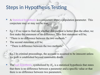
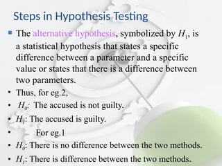
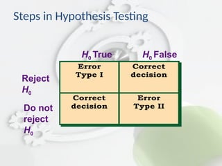
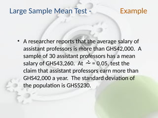
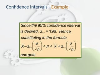
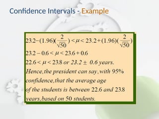
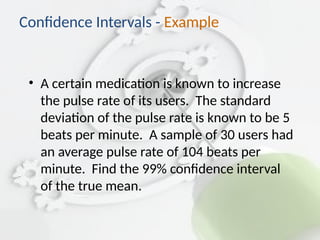
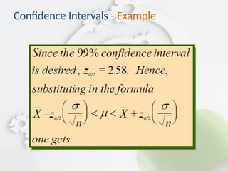
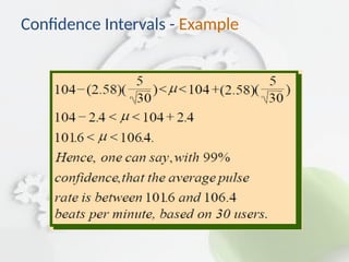
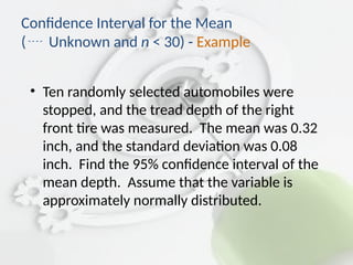
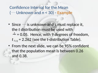
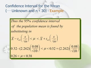
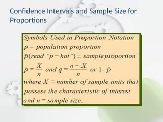
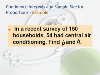
A Statistical hypothesis is a conjecture about a population parameter. This conjecture may or may not be true.
Eg.1 If we want to find out whether one method is better than the other, we first make the statement of no difference. This first statement will be;
“There is no difference between the two methods.”
The second statement will be;
“There is difference between the two methods.”
Eg.2 In criminal proceedings, the accused is assumed to be innocent unless his guilt is established beyond reasonable doubt.
The null hypothesis, symbolized by H0, is a statistical hypothesis that states that there is no difference between a parameter and a specific value or that there is no difference between two parameters.


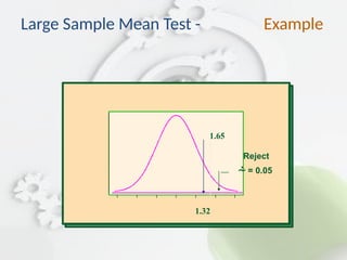
![ Step 3: z = [43,260 – 42,000]/[5230/30] =
1.32.
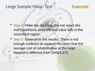
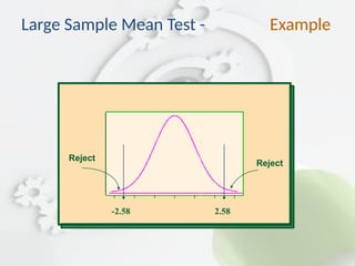
Step 4: Make the decision. Since the test value,
+1.32, is less than the critical value, +1.65, and
not in the critical region, the decision is “Do not
reject the null hypothesis.”
Large Sample Mean Test - Example](https://image.slidesharecdn.com/hypothesistestingconfidenceinterval-250915115146-86dafed7/85/Hypothesis-Testing-Confidence-Interval-pptx-26-320.jpg)
![ Step 3: z = [27– 29.4]/[2/30] = –6.57.
Step 4: Make the decision. Since the test value,
–6.57, falls in the critical region, the decision is
to reject the null hypothesis.
Large Sample Mean Test - Example](https://image.slidesharecdn.com/hypothesistestingconfidenceinterval-250915115146-86dafed7/85/Hypothesis-Testing-Confidence-Interval-pptx-31-320.jpg)
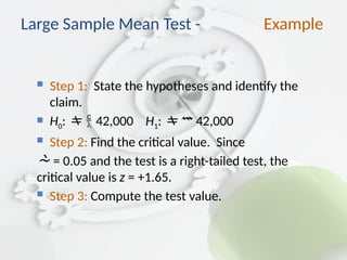
![ Step 2: Find the critical values. Since =
0.01 and the test is a two-tailed test, the critical
values are z = –2.58 and +2.58.
Step 3: Compute the test value.
Step 3: z = [25,226 – 24,672]/[3,251/35] =
1.01.
Large Sample Mean Test - Example](https://image.slidesharecdn.com/hypothesistestingconfidenceinterval-250915115146-86dafed7/85/Hypothesis-Testing-Confidence-Interval-pptx-36-320.jpg)
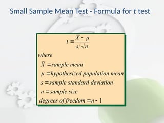
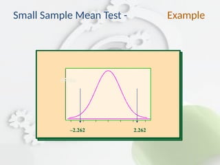
![ Step 3: Compute the test value.
t = [23,450 – 24,000]/[400/] = – 4.35.
Step 4: Reject the null hypothesis, since
– 4.35 < – 2.262.
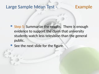
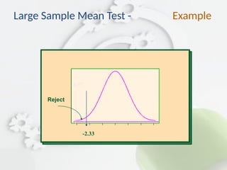
Step 5: There is enough evidence to reject the
claim that the starting salary of nurses is
24,000.
Small Sample Mean Test - Example](https://image.slidesharecdn.com/hypothesistestingconfidenceinterval-250915115146-86dafed7/85/Hypothesis-Testing-Confidence-Interval-pptx-45-320.jpg)
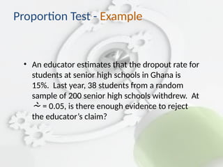
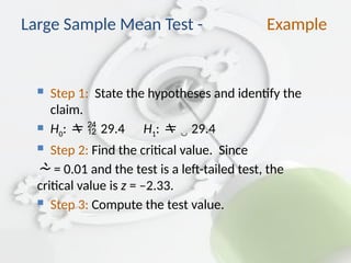
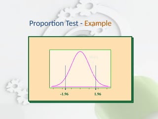
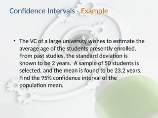
![ Step 1: State the hypotheses and identify the claim.
H0: p0.15 H1: p 0.15
Step 2: Find the mean and standard deviation. =
np = (200)(0.15) = 30 and
= [
(200)(0.15)(0.85)] = 5.05.
Step 3: Find the critical values. Since
= 0.05 and the test is two-tailed the critical
values are z = 1.96.
Proportion Test - Example](https://image.slidesharecdn.com/hypothesistestingconfidenceinterval-250915115146-86dafed7/85/Hypothesis-Testing-Confidence-Interval-pptx-50-320.jpg)
![ Step 4: Compute the test value. z =
[38 – 30]/[5.05] = 1.58.
Step 5: Do not reject the null hypothesis,
since the test value falls outside the critical
region.
Proportion Test - Example](https://image.slidesharecdn.com/hypothesistestingconfidenceinterval-250915115146-86dafed7/85/Hypothesis-Testing-Confidence-Interval-pptx-51-320.jpg)
![Outline
• Introduction
• Confidence Intervals for the Mean [
Known or n 30] and Sample Size
• Confidence Intervals for the Mean [
Unknown and n 30]](https://image.slidesharecdn.com/hypothesistestingconfidenceinterval-250915115146-86dafed7/85/Hypothesis-Testing-Confidence-Interval-pptx-55-320.jpg)


![MATH 564 Advanced Mathematics for Data Science[1].pptx](https://cdn.slidesharecdn.com/ss_thumbnails/math564advancedmathematicsfordatascience1-250915112031-c023a536-thumbnail.jpg?width=640&height=640&fit=bounds)


