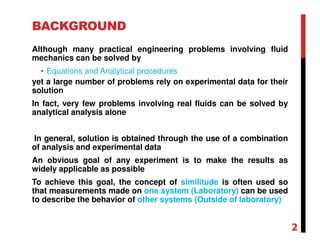
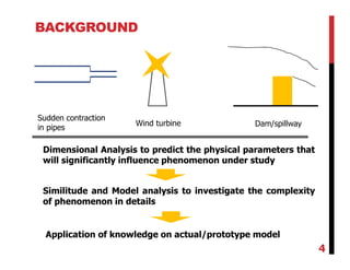
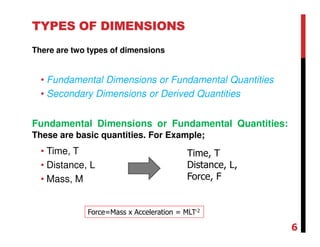
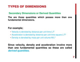
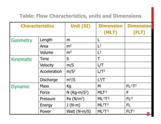
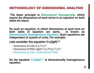
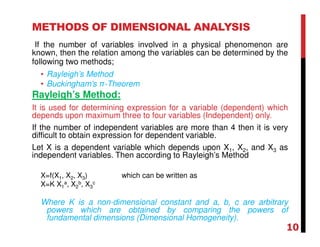
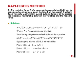
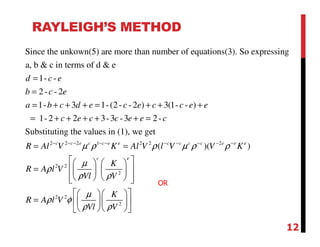
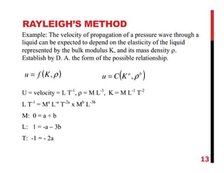
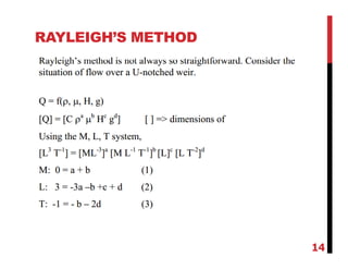
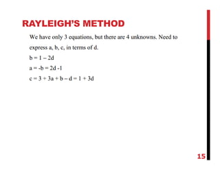
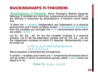
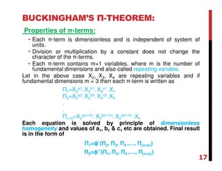
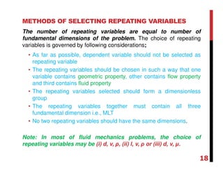
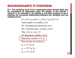
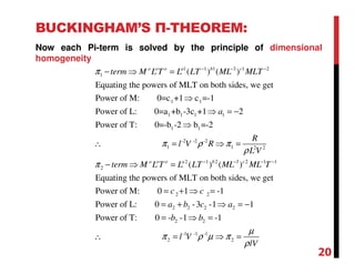
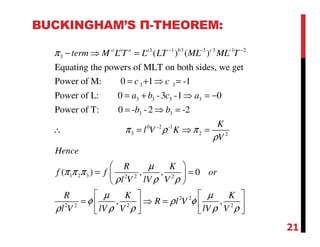
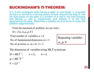
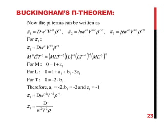
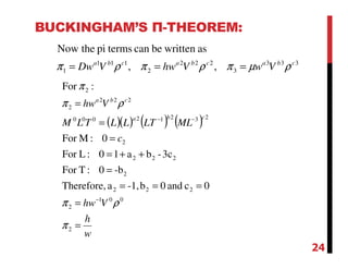
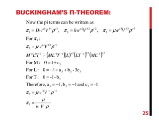
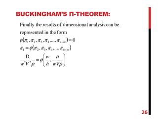
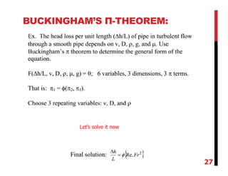
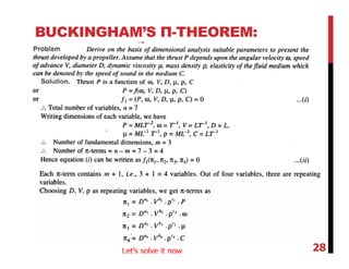
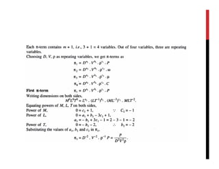
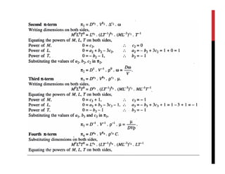
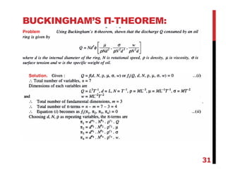
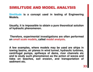
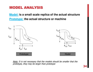
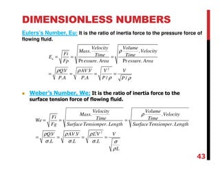
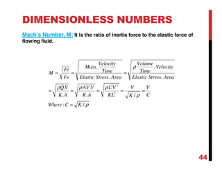
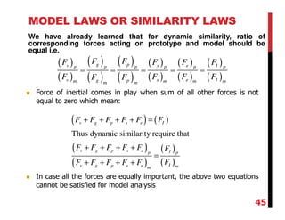
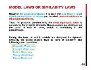
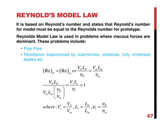
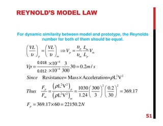
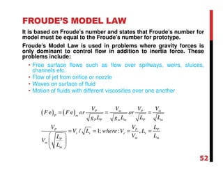
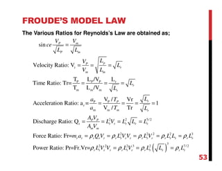
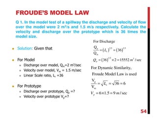
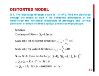
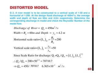
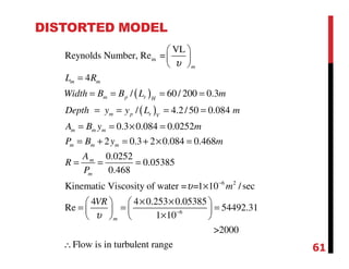
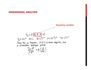
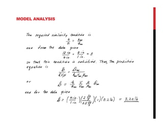
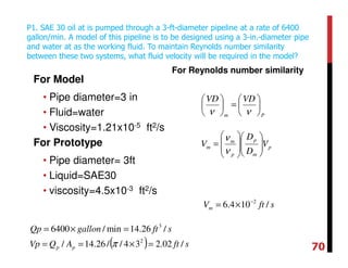
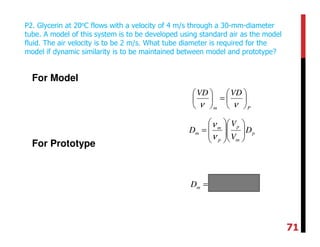
The document discusses dimensional analysis, similitude, and model analysis. It provides background on how dimensional analysis and model testing are used to study fluid mechanics problems. Dimensional analysis uses the dimensions of physical quantities to determine which parameters influence a phenomenon. Model testing in a laboratory allows measurements to be applied to larger scale systems using similitude. Buckingham's π-theorem is introduced as a way to non-dimensionalize variables when there are more variables than fundamental dimensions. Rayleigh's and Buckingham's methods are demonstrated on an example of determining the resisting force on an aircraft.

1. DIMENSIONAL ANALYSIS,
SIMILITUDE AND MODEL
ANALYSIS
DR. MOHSIN SIDDIQUE
ASSISTANT PROFESSOR

2. BACKGROUND
Although many practical engineering problems involving fluid
mechanics can be solved by
• Equations and Analytical procedures
yet a large number of problems rely on experimental data for their
solution
In fact, very few problems involving real fluids can be solved by
analytical analysis alone
In general, solution is obtained through the use of a combination
of analysis and experimental data
An obvious goal of any experiment is to make the results as
widely applicable as possible
To achieve this goal, the concept of similitude is often used so
that measurements made on one system (Laboratory) can be used
to describe the behavior of other systems (Outside of laboratory)
2

3. BACKGROUND
The laboratory systems are usually thought of as models
and are used to study the phenomenon of interest under
carefully controlled conditions
From these model studies, empirical formulations can be
developed, or specific predictions of one or more
characteristics of some other similar system can be made
However, to do this, it is necessary to establish the
relationship between the laboratory model and the “other”
system
In present topic, we will learn how to achieve this in a
systematic manner
3

4. BACKGROUND
Dimensional Analysis to predict the physical parameters that
will significantly influence phenomenon under study
Similitude and Model analysis to investigate the complexity
of phenomenon in details
Application of knowledge on actual/prototype model
Wind turbine Dam/spillway
Sudden contraction
in pipes
4

5. DIMENSIONAL ANALYSIS
Introduction:
Dimensional Analysis is a mathematical technique making
use of study of dimensions
It deals with the dimensions of physical quantities involved
in the phenomenon
In dimensional analysis, one first predicts the physical
parameters that will influence the flow, and then by,
grouping these parameters in dimensionless combinations
a better understanding of the flow phenomenon is made
possible
It is particularly helpful in experimental work because it
provides a guide to those things that significantly influence
the phenomena; thus it indicates the direction in which the
experimental work should go
This mathematical technique is used in research work for
design and for conducting model tests
5

6. TYPES OF DIMENSIONS
There are two types of dimensions
• Fundamental Dimensions or Fundamental Quantities
• Secondary Dimensions or Derived Quantities
Fundamental Dimensions or Fundamental Quantities:
These are basic quantities. For Example;
• Time, T
• Distance, L
• Mass, M
Time, T
Distance, L,
Force, F
Force=Mass x Acceleration = MLT-2
6

7. TYPES OF DIMENSIONS
Secondary Dimensions or Derived Quantities
The are those quantities which posses more than one
fundamental dimensions.
For example;
• Velocity is denoted by distance per unit time L/T
• Acceleration is denoted by distance per unit time square L/T2
• Density is denoted by mass per unit volume M/L3
Since velocity, density and acceleration involve more
than one fundamental quantities so these are called
derived quantities.
7

8. Characteristics Unit (SI) Dimension
(MLT)
Dimension
(FLT)
Geometry Length m L
Area m2 L2
Volume m3 L3
Kinematic Time S T
Velocity m/S L/T
Acceleration m/S2 L/T2
Discharge m3/S L3/T
Dynamic Mass Kg M FL-1T2
Force N (Kg-m/S2) MLT-2 F
Pressure Pa (N/m2) ML-1T-2 FL-2
Energy J (N-m) ML2T-2 FL
Power Watt (N-m/S) ML2T-3 FLT-1
Table: Flow Characteristics, units and Dimensions
8

9. METHODOLOGY OF DIMENSIONAL ANALYSIS
The basic principle is Dimensional Homogeneity, which
means the dimensions of each terms in an equation on both
sides are equal.
So such an equation, in which dimensions of each term on
both sides of equation are same, is known as
Dimensionally Homogeneous Equation. Such equations are
independent of system of units. For example;
Lets consider the equation V=(2gH)1/2
• Dimensions of LHS=V=L/T=LT-1
• Dimensions of RHS=(2gH)1/2=(L/T2xL)1/2=LT-1
• Dimensions of LHS = Dimensions of RHS
So the equation V=(2gH)1/2 is dimensionally homogeneous
equation.
9

10. METHODS OF DIMENSIONAL ANALYSIS
If the number of variables involved in a physical phenomenon are
known, then the relation among the variables can be determined by the
following two methods;
• Rayleigh’s Method
• Buckingham’s π-Theorem
Rayleigh’s Method:
It is used for determining expression for a variable (dependent) which
depends upon maximum three to four variables (Independent) only.
If the number of independent variables are more than 4 then it is very
difficult to obtain expression for dependent variable.
Let X is a dependent variable which depends upon X1, X2, and X3 as
independent variables. Then according to Rayleigh’s Method
X=f(X1, X2, X3) which can be written as
X=K X1
a, X2
b, X3
c
Where K is a non-dimensional constant and a, b, c are arbitrary
powers which are obtained by comparing the powers of
fundamental dimensions (Dimensional Homogeneity).
10

11. RAYLEIGH’S METHOD
Q. The resisting force R of a supersonic plane during flight can be
considered as dependent upon the length of the aircraft l, velocity
V, air viscosity µ, air density ρ, and bulk modulus of air k. Express
the functional relationship between the variables and the resisting
force.
-2 1 1 1 3 1 2
( , , , , ) , , , , (1)
Where: A = Non dimensional constant
Substituting the powers on both sides of the equation
( ) ( ) ( ) ( )
Equating the powers of MLT on both
a b c d e
a b c d e
R f l V K R Al V K
MLT AL LT ML T ML ML T
µ ρ µ ρ
− − − − − −
= ⇒ =
=
sides
Power of M 1
Power of L 1 - -3 -
Power of T 2 - - -2
c d e
a b c d e
b c e
⇒ = + +
⇒ = +
⇒ − =
Solution:
11

12. RAYLEIGH’S METHOD
Since the unkown(5) are more than number of equations(3). So expressing
a, b & c in terms of d & e
1- -
2- - 2
1- 3 1-(2- - 2 ) 3(1- - )
1-2 2 3-3 -3 2-
Substituting the values
d c e
b c e
a b c d e c e c c e e
c e c c e e c
=
=
= + + + = + + +
= + + + + + =
2 2 2 1 2 2 2
2 2
2
2 2
2
in (1), we get
( )( )c c e c c e e c c c c e e e
c e
R Al V K Al V l V V K
K
R A l V
Vl V
K
R A l V
Vl V
µ ρ ρ µ ρ ρ
µ
ρ
ρ ρ
µ
ρ φ
ρ ρ
− − − − − − − − − −
= =
    
=     
     
   
=    
   
OR
12

13. RAYLEIGH’S METHOD
( )ρ,Kfu = ( )ba
KCu ρ,=
13

14. RAYLEIGH’S METHOD
14

15. RAYLEIGH’S METHOD
15

16. BUCKINGHAM’S Π-THEOREM:
Buckingham’s π-Theorem: Since Rayleigh’s Method becomes
laborious if variables are more than fundamental dimensions (MLT), so
the difficulty is overcome by Buckingham’s π-Theorem which states
that
“If there are n variables (Independent and Dependent) in a physical
phenomenon and if these variables contain m fundamental dimensions
then the variables are arranged into (n-m) dimensionless terms which
are called π-terms.”
Let X1, X2, X3,…,X4, Xn are the variables involved in a physical
problem. Let X1 be the dependent variable and X2, X3, X4,…,Xn are
the independent variables on which X1 depends. Mathematically it can
be written as
X1=f(X2 ,X3 ,X4 ,Xn) which can be rewritten as
f(X1X2 ,X3 ,X4 ,Xn)=0
Above equation is dimensionally homogenous.
It contain n variables and if there are m fundamental dimensions then it
can be written in terms of dimensions groups called π-terms which are
equal to (n-m)
Hence; f(π1, π2 π3,… πn-m)=0
16

17. BUCKINGHAM’S Π-THEOREM:
Properties of π-terms:
• Each π-term is dimensionless and is independent of system of
units.
• Division or multiplication by a constant does not change the
character of the π-terms.
• Each π-term contains m+1 variables, where m is the number of
fundamental dimensions and also called repeating variable.
Let in the above case X2, X3, X4 are repeating variables and if
fundamental dimensions m = 3 then each π-term is written as
Π1=X2
a1. X3
b1. X4
c1 .X1
Π2=X2
a2. X3
b2. X4
c2 .X5
.
.
Πn-m=X2
a(n-m). X3
b(n-m). X4
a(n-m) .Xn
Each equation is solved by principle of dimensionless
homogeneity and values of a1, b1 & c1 etc are obtained. Final result
is in the form of
Π1=ϕ’(Π2, Π3, Π4 ,…, Π(n-m))
Π2=ϕ”(Π1, Π3, Π4 ,…, Π(n-m))
17

18. METHODS OF SELECTING REPEATING VARIABLES
The number of repeating variables are equal to number of
fundamental dimensions of the problem. The choice of repeating
variables is governed by following considerations;
• As far as possible, dependent variable should not be selected as
repeating variable
• The repeating variables should be chosen in such a way that one
variable contains geometric property, other contains flow property
and third contains fluid property
• The repeating variables selected should form a dimensionless
group
• The repeating variables together must contain all three
fundamental dimension i.e., MLT
• No two repeating variables should have the same dimensions.
Note: In most of fluid mechanics problems, the choice of
repeating variables may be (i) d, v, ρ, (ii) l, v, ρ or (iii) d, v, µ.
18

19. BUCKINGHAM’S Π-THEOREM:
Q 1. The resisting force R of a supersonic plane during flight can
be considered as dependent upon the length of the aircraft l,
velocity V, air viscosity µ, air density ρ, and bulk modulus of air k.
Express the functional relationship between the variables and the
resisting force.
1 2 3
( , , , , ) ( , , , , , ) 0
Total number of variables, n= 6
No. of fundamental dimension, m=3
No. of dimensionless -terms, n-m=3
Thus: ( , , ) 0
No. Repeating variables =m=3
Repeating variables = ,
R f l V K f R l V K
f
l
µ ρ µ ρ
π
π π π
= ⇒ =
=
1 1 1
1
2 2 2
2
3 3 3
3
,
π-terms are written as
a b c
a b c
a b c
V
Thus
l V R
l V
l V K
ρ
π ρ
π ρ µ
π ρ
=
=
=
19

20. BUCKINGHAM’S Π-THEOREM:
Now each Pi-term is solved by the principle of dimensional
homogeneity
1 1 1 3 1 2
1
1 1
1 1 1 1
1 1
( ) ( )
Equating the powers of MLT on both sides, we get
Power of M: 0=c +1 c =-1
Power of L: 0=a +b -3c +1 2
Power of T: 0=-b -2 b =-2
o o o a b c
term M L T L LT ML MLT
a
π − − −
− ⇒ =
⇒
⇒ = −
⇒
∴ -2 -2 -2
1 1 2 2
2 1 2 3 2 1 1
2
2 2
2 2 2 2
( ) ( )
Equating the powers of MLT on both sides, we get
Power of M: 0 1 -1
Power of L: 0 -3 -1 1
Pow
o o o a b c
R
l V R
L V
term M L T L LT ML ML T
c c
a b c a
π ρ π
ρ
π − − − −
= ⇒ =
− ⇒ =
= + ⇒ =
= + ⇒ = −
2 2
-1 -1 -1
2 2
er of T: 0 - -1 -1b b
l V
lV
µ
π ρ µ π
ρ
= ⇒ =
∴ = ⇒ =
20

21. BUCKINGHAM’S Π-THEOREM:
3 1 3 3 3 1 2
3
3 3
3 3 3 3
3 3
( ) ( )
Equating the powers of MLT on both sides, we get
Power of M: 0 1 -1
Power of L: 0 -3 -1 0
Power of T: 0 - - 2 -2
o o o a b c
term M L T L LT ML ML T
c c
a b c a
b b
π − − − −
− ⇒ =
= + ⇒ =
= + ⇒ = −
= ⇒ =
∴ 0 -2 -1
3 2 2
1 2 3 2 2 2
2 2
2 2 2 2
( ) , , 0
, ,
K
l V K
V
Hence
R K
f f or
l V lV V
R K K
R l V
l V lV V lV V
π ρ π
ρ
µ
π π π
ρ ρ ρ
µ µ
φ ρ φ
ρ ρ ρ ρ ρ
= ⇒ =
 
= = 
 
   
= ⇒ =   
   
21

22. BUCKINGHAM’S Π-THEOREM:
Q 2. A thin rectangular plate having a width, w, and height, h, is located
so that it is normal to a moving stream of fluid. Assume the drag D, that
the fluid exerts on the plate is a function of w and h, the fluid viscosity
and density µ, and ρ, respectively, and velocity V of the fluid
approaching the plate. Determine a suitable set of pi terms to study this
problem experimentally
( )Vhwf ,,,,D
:can writeweproblem,ofstatementtheFrom
ρµ=
33-6m-nterms,piofNo.
3mdimension,lfundamentaofNo.
6n,variablesofnumberTotal
==
=
=
V,w,
variablesRepeating
ρ
1
11
2
,,D
aresystemMLTusingvariablesofdimensionThe
−
−−
=
=
===
LTV
TML
LhLwMLT -
µ
22

23. BUCKINGHAM’S Π-THEOREM:
333
3
222
2
111
1 ,,
aswrittenbecantermspitheNow
cbacbacba
VwVhwVDw ρµπρπρπ ===
( )( ) ( ) ( )
ρ
π
ρπ
ρπ
π
221
122
1
111
1
111
1
131112000
111
1
1
D
D
-1cand-2b-2,aTherefore,
b--20:TFor
3c-ba10:LFor
10:MFor
D
:For
Vw
Vw
c
MLLTLMLTTLM
Vw
cba
cba
=
=
===
=
++=
+=
=
=
−−−
−−−
23

24. BUCKINGHAM’S Π-THEOREM:
333
3
222
2
111
1 ,,
aswrittenbecantermspitheNow
cbacbacba
VwVhwVDw ρµπρπρπ ===
( )( ) ( ) ( )
w
h
Vhw
c
MLLTLLTLM
Vhw
cba
cba
=
=
===
=
++=
=
=
=
−
−−
2
001
2
222
2
222
2
23212000
222
2
2
0cand0b-1,aTherefore,
-b0:TFor
3c-ba10:LFor
0:MFor
:For
π
ρπ
ρπ
π
24

25. BUCKINGHAM’S Π-THEOREM:
333
3
222
2
111
1 ,,
aswrittenbecantermspitheNow
cbacbacba
VwVhwVDw ρµπρπρπ ===
( )( ) ( ) ( )
ρ
µ
π
ρµπ
ρµπ
π
Vw
Vw
c
MLLTLTMLTLM
Vw
cba
cba
=
=
=−=−=
=
++−=
+=
=
=
−−−
−−−−
3
111
3
333
3
333
3
3331311000
333
3
3
-1cand1b1,aTherefore,
b--10:TFor
3c-ba10:LFor
10:MFor
:For
25

26. BUCKINGHAM’S Π-THEOREM:
( )
( )






=
=
=
−
−
ρ
µ
φ
ρ
ππππφπ
πππππφ
wVh
w
Vw
mn
mn
,
D
,...,,,
0,...,,,,
formin thedrepresente
becananalysisldimensionaofresultseFinally th
22
4321
4321
26

27. BUCKINGHAM’S Π-THEOREM:
27
Let’s solve it now

28. BUCKINGHAM’S Π-THEOREM:
28Let’s solve it now

31. BUCKINGHAM’S Π-THEOREM:
31

32. For more worked problems refer to
Civil Engineering Hydraulics by Nalluri and Featherstone
(Worked problems 9.1 to 9.11)

33. SIMILITUDE AND MODEL ANALYSIS
Similitude is a concept used in testing of Engineering
Models.
Usually, it is impossible to obtain a pure theoretical solution
of hydraulic phenomenon.
Therefore, experimental investigations are often performed
on small scale models, called model analysis.
A few examples, where models may be used are ships in
towing basins, air planes in wind tunnel, hydraulic turbines,
centrifugal pumps, spillways of dams, river channels etc
and to study such phenomenon as the action of waves and
tides on beaches, soil erosion, and transportation of
sediment etc.
33

34. MODEL ANALYSIS
Model: is a small scale replica of the actual structure
Prototype: the actual structure or machine
Prototype Model
Lp3
Lp1
Lp2
Fp1
Fp3
Fp2
Lm3
Lm1
Lm2
Fm1
Fm3
Fm2
34
Note: It is not necessary that the models should be smaller that the
prototype, they may be larger than prototype

35. MODEL ANALYSIS
Model Analysis is actually an experimental method of
finding solutions of complex flow problems
The followings are the advantages of the model analysis
• Using dimensional analysis, a relationship between the
variables influencing a flow problem is obtained which help in
conducting tests
• The performance of the hydraulic structure can be predicted
in advance from its model
• The merits of alternative design can be predicted with the
help of model analysis to adopt most economical, and safe
design
Note: Test performed on models can be utilized for
obtaining, in advance, useful information about the
performance of the prototype only if a complete similarity
exits between the model and the prototype
35

36. SIMILITUDE-TYPE OF SIMILARITIES
Similitude: is defined as similarity between the model
and prototype in every respect, which mean model and
prototype have similar properties or model and
prototype are completely similar.
Three types of similarities must exist between model
and prototype.
• Geometric Similarity
• Kinematic Similarity
• Dynamic Similarity
36

37. SIMILITUDE-TYPE OF SIMILARITIES
Geometric Similarity: is the similarity of shape. It is said to exist
between model and prototype if ratio of all the corresponding
linear dimensions in the model and prototype are equal. e.g.
p p p
r
m m m
L B D
L
L B D
= = =
Where: Lp, Bp and Dp are Length, Breadth, and diameter of prototype
and Lm, Bm, Dm are Length, Breadth, and diameter of model.
Lr= Scale ratio
Note: Models are generally prepared with same scale ratios in every
direction. Such models are called true models. However, sometimes
it is not possible to do so and different convenient scales are used in
different directions. Thus, such models are called distorted model
37

38. SIMILITUDE-TYPE OF SIMILARITIES
Kinematic Similarity: is the similarity of motion. It is said to exist
between model and prototype if ratio of velocities and acceleration
at the corresponding points in the model and prototype are equal.
e.g.
1 2 1 2
1 2 1 2
;
p p p p
r r
m m m m
V V a a
V a
V V a a
= = = =
Where: Vp1& Vp2 and ap1 & ap2 are velocity and accelerations at point
1 & 2 in prototype and Vm1& Vm2 and am1 & am2 are velocity and
accelerations at point 1 & 2 in model.
Vr and ar are the velocity ratio and acceleration ratio
Note: Since velocity and acceleration are vector quantities, hence
not only the ratio of magnitude of velocity and acceleration at the
corresponding points in model and prototype should be same; but
the direction of velocity and acceleration at the corresponding points
in model and prototype should also be parallel.
38

39. SIMILITUDE-TYPE OF SIMILARITIES
Dynamic Similarity: is the similarity of forces. It is said to exist
between model and prototype if ratio of forces at the
corresponding points in the model and prototype are equal. e.g.
( )
( )
( )
( )
( )
( )
gi vp p p
r
i v gm m m
FF F
F
F F F
= = =
Where: (Fi)p, (Fv)p and (Fg)p are inertia, viscous and gravitational
forces in prototype and (Fi)m, (Fv)m and (Fg)m are inertia, viscous and
gravitational forces in model.
Fr is the Force ratio
Note: The direction of forces at the corresponding points in model
and prototype should also be parallel.
39

40. TYPES OF FORCES ENCOUNTERED IN FLUID
PHENOMENON
Inertia Force, Fi: It is equal to product of mass and acceleration in the
flowing fluid.
Viscous Force, Fv: It is equal to the product of shear stress due to
viscosity and surface area of flow.
Gravity Force, Fg: It is equal to product of mass and acceleration due
to gravity.
Pressure Force, Fp: it is equal to product of pressure intensity and
cross-sectional area of flowing fluid.
Surface Tension Force, Fs: It is equal to product of surface tension
and length of surface of flowing fluid.
Elastic Force, Fe: It is equal to product of elastic stress and area of
flowing fluid.
40

41. DIMENSIONLESS NUMBERS
Dimensionless numbers are the numbers which are
obtained by dividing the inertia force by viscous force or
gravity force or pressure force or surface tension force or
elastic force.
As this is ratio of once force to other, it will be a
dimensionless number. These are also called non-
dimensional parameters.
The following are most important dimensionless numbers.
• Reynold’s Number
• Froude’s Number
• Euler’s Number
• Weber’s Number
• Mach’s Number
41

42. DIMENSIONLESS NUMBERS
Reynold’s Number, Re: It is the ratio of inertia force to the viscous force
of flowing fluid.
. .
Re
. .
. . .
. . .
Velocity Volume
Mass Velocity
Fi Time Time
Fv Shear Stress Area Shear Stress Area
QV AV V AV V VL VL
du VA A A
dy L
ρ
ρ ρ ρ ρ
τ µ υµ µ
= = =
= = = = =
2
. .
. .
. .
. .
Velocity Volume
Mass Velocity
Fi Time TimeFe
Fg Mass Gavitational Acceleraion Mass Gavitational Acceleraion
QV AV V V V
Volume g AL g gL gL
ρ
ρ ρ
ρ ρ
= = =
= = = =
Froude’s Number, Fe: It is the ratio of inertia force to the gravity force
of flowing fluid.
42

43. DIMENSIONLESS NUMBERS
Eulers’s Number, Eu: It is the ratio of inertia force to the pressure force of
flowing fluid.
2
. .
Pr . Pr .
. .
. . / /
u
Velocity Volume
Mass Velocity
Fi Time TimeE
Fp essure Area essure Area
QV AV V V V
P A P A P P
ρ
ρ ρ
ρ ρ
= = =
= = = =
2 2
. .
. .
. .
. . .
Velocity Volume
Mass Velocity
Fi Time TimeWe
Fg Surface Tensionper Length Surface Tensionper Length
QV AV V L V V
L L L
L
ρ
ρ ρ ρ
σ σ σ σ
ρ
= = =
= = = =
Weber’s Number, We: It is the ratio of inertia force to the
surface tension force of flowing fluid.
43

44. DIMENSIONLESS NUMBERS
Mach’s Number, M: It is the ratio of inertia force to the elastic force of
flowing fluid.
2 2
2
. .
. .
. .
. . /
: /
Velocity Volume
Mass Velocity
Fi Time TimeM
Fe Elastic Stress Area Elastic Stress Area
QV AV V L V V V
K A K A KL CK
Where C K
ρ
ρ ρ ρ
ρ
ρ
= = =
= = = = =
=
44

45. MODEL LAWS OR SIMILARITY LAWS
We have already learned that for dynamic similarity, ratio of
corresponding forces acting on prototype and model should be
equal i.e.
( )
( )
( )
( )
( )
( )
( )
( )
( )
( )
( )
( )
g pv s e Ip p p p p p
v s e Ig pm m m mm m
F FF F F F
F F F FF F
= = = = =
( ) ( )
( )
( )
( )
( )
Thus dynamic similarity require that
v g p s e I
v g p s e Ip p
Iv g p s e mm
F F F F F F
F F F F F F
FF F F F F
+ + + + =
+ + + +
=
+ + + +
Force of inertial comes in play when sum of all other forces is not
equal to zero which mean:
In case all the forces are equally important, the above two equations
cannot be satisfied for model analysis
45

46. MODEL LAWS OR SIMILARITY LAWS
However, for practical problems it is seen that one force is most
significant compared to others and is called predominant force or
most significant force.
Thus, for practical problem only the most significant force is
considered for dynamic similarity. Hence, models are designed on
the basis of ratio of force, which is dominating in the
phenomenon.
Finally, the laws on which models are designed for dynamic
similarity are called models laws or laws of similarity. The
followings are these laws
• Reynold’s Model Law
• Froude’s Model Law
• Euler’s Model Law
• Weber’s Model Law
• Mach’s Model Law
46

47. REYNOLD’S MODEL LAW
It is based on Reynold’s number and states that Reynold’s number
for model must be equal to the Reynolds number for prototype.
Reynolds Model Law is used in problems where viscous forces are
dominant. These problems include:
• Pipe Flow
• Resistance experienced by submarines, airplanes, fully immersed
bodies etc
( ) ( )Re Re
1
: , ,
m mP P
P m
P m
P P r r
rP
m m
m
P P P
r r r
m m m
V LV L
or
V L V L
V L
V L
where V L
V L
υ υ
υυ
υ
υ
υ
υ
= =
= =
 
 
 
= = =
47

48. REYNOLD’S MODEL LAW
The Various Ratios for Reynolds’s Law are obtained as
r
r
r
P P P r
m m m r
P P
r
m m
2
r
r
sin /
Velocity Ratio: V =
L
T L /V L
Time Ratio: Tr=
T L /V V
V / Vr
Acceleration Ratio: a =
V / Tr
Discharge Ratio: Q
Force Ratio: F =
P m
mP P
m P m
P
m
P P
r r
m m
VL VL
ce and
LV
V L
a T
a T
A V
L V
A V
m
υ µ ρ
υ υ
υ υ
υ
   
= =   
   
= =
= =
= =
= =
2 2 2
2 2 2 3
r r rPower Ratio: P =F .V =
r r r r r r r r r r r r
r r r r r r r
a Q V L V V L V
L V V L V
ρ ρ ρ
ρ ρ
= = =
=
48

49. REYNOLD’S MODEL LAW
Q. A pipe of diameter 1.5 m is required to transport an oil of specific
gravity 0.90 and viscosity 3x10-2 poise at the rate of 3000litre/s.
Tests were conducted on a 15 cm diameter pipe using water at
20oC. Find the velocity and rate of flow in the model.
p p p p pm m m
m m
2
2
p 2
For pipe flow,
According to Reynolds' Model Law
V D DV D
D
900 1.5 1 10
3.0
1000 0.15 3 10
3.0
Since V
/ 4(1.5)
1.697 /
3.0 5.091 /
5.
m m
m p p p
m
p
p
p
m p
m m m
V
V
V
V
Q
A
m s
V V m s
and Q V A
ρ ρ µρ
µ µ ρ µ
π
−
−
= ⇒ =
× ×
= =
× ×
= =
=
∴ = =
= = 2
3
091 / 4(0.15)
0.0899 /m s
π×
=
Solution:
Prototype Data:
Diameter, Dp= 1.5m
Viscosity of fluid, µp= 3x10-2 poise
Discharge, Qp =3000litre/sec
Sp. Gr., Sp=0.9
Density of oil=ρp=0.9x1000
=900kg/m3
Model Data:
Diameter, Dm=15cm =0.15 m
Viscosity of water, µm =1x10-2 poise
Density of water, ρm=1000kg/m3
Velocity of flow Vm=?
Discharge Qm=?
49

50. REYNOLD’S MODEL LAW
Q. A ship 300m long moves in sea water, whose density is 1030
kg/m3. A 1:100 model of this ship is to be tested in a wind tunnel.
The velocity of air in the wind tunnel around the model is 30m/s and
the resistance of the model is 60N.
Determine the velocity of ship in sea water and also the resistance
of ship in sea water. The density of air is given as 1.24kg/m3. Take
the kinematic viscosity of air and sea water as 0.012 stokes and
0.018 stokes respectively.
Solution:
For Prototype
Length, Lp= 300m
Fluid = sea water
Density of sea water, ρp= 1030 kg/m3
Kinematic Viscosity, νp=0.018 stokes
=0.018x10-4 m2/s
Let Velocity of ship, Vp
Resistance, Fp
For Model
Scale ratio = Lp/Lm=100
Length, Lm= Lp/100 = 3m
Fluid = air
Density of air, ρm= 1.24 kg/m3
Kinematic Viscosity, νm=0.012 stokes
=0.012x10-4 m2/s
Velocity of ship, Vm=30 m/s
Resistance, Fm = 60 N
50

51. ( )
( )
4
4
2 2
2 2 2 2
2 2
0.012 10 3
30 0.2 /
0.018 10 300
Resistance= Mass Acceleration= L V
L V 1030 300 0.2
369.17
1.24 3 30L V
369.17 60 22150.2
p m
p m
p m m p
p p
m
m
p
LVL VL
V V
L
Vp m s
Since
F
Thus
F
F N
υ
υ υ υ
ρ
ρ
ρ
−
−
   
= ⇒ =   
   
×
= =
×
×
   
= = =   
   
= × =
REYNOLD’S MODEL LAW
For dynamic similarity between model and prototype, the Reynolds
number for both of them should be equal.
51
0.018
0.012

52. FROUDE’S MODEL LAW
It is based on Froude’s number and states that Froude’s number for
model must be equal to the Froude’s number for prototype.
Froude’s Model Law is used in problems where gravity forces is
only dominant to control flow in addition to inertia force. These
problems include:
• Free surface flows such as flow over spillways, weirs, sluices,
channels etc.
• Flow of jet from orifice or nozzle
• Waves on surface of fluid
• Motion of fluids with different viscosities over one another
( ) ( )e e
/ 1; : ,
m mP P
P m
P P m m P m
P P P
r r r r
m mP
m
m
V VV V
F F or or
g L g L L L
V V L
V L where V L
V LL
V
L
= = =
= = = =
 
 
 
52

53. FROUDE’S MODEL LAW
The Various Ratios for Reynolds’s Law are obtained as;
r
P P P r
m m m
P P
r
m m
2 2 5/ 2
r
sin
Velocity Ratio: V
T L /V L
Time Ratio: Tr=
T L /V
V / Vr
Acceleration Ratio: a = 1
V / Tr
Discharge Ratio: Q
Force Ratio: Fr=
mP
P m
pP
r
m m
r
r
rP
m r
P P
r r r r r
m m
r r
VV
ce
L L
LV
L
V L
L
L
La T
a T L
A V
L V L L L
A V
m a
=
= = =
= = =
= = = =
= = = =
=
( )
2 2 2 2 3
3
2 2 2 3 2 7/ 2
Power Ratio: Pr=Fr.Vr=
r r r r r r r r r r r r r r r
r r r r r r r r r r r r
Q V L V V L V L L L
L V V L V L L L
ρ ρ ρ ρ ρ
ρ ρ ρ ρ
= = = =
= = =
53

54. FROUDE’S MODEL LAW
Q 1. In the model test of a spillway the discharge and velocity of flow
over the model were 2 m3/s and 1.5 m/s respectively. Calculate the
velocity and discharge over the prototype which is 36 times the
model size.
( ) ( )
( )
2.5 2.5p
m
2.5 3
For Discharge
Q
36
Q
36 2 15552 /sec
r
p
L
Q m
= =
= × =
p
m
For Dynamic Similarity,
Froude Model Law is used
V
36 6
V
6 1.5 9 /sec
r
p
L
V m
= = =
= × =
Solution: Given that
For Model
Discharge over model, Qm=2 m3/sec
Velocity over model, Vm = 1.5 m/sec
Linear Scale ratio, Lr =36
For Prototype
Discharge over prototype, Qp =?
Velocity over prototype Vp=?
54

55. FROUDE’S MODEL LAW
Q 2. The characteristics of the spillway are to be studied by means of a geometrically
similar model constructed to a scale of 1:10.
(i) If 28.3 cumecs, is the maximum rate of flow in prototype, what will be the
corresponding flow in model?
(i) If 2.4m/s, 50mm and 3.5 Nm are values of velocity at a point on the spillway, height
of hydraulic jump and energy dissipated per second in model, what will be the
corresponding velocity, height of hydraulic jump and energy dissipation per second in
prototype?
Solution: Given that
For Model
Discharge over model, Qm=?
Velocity over model, Vm = 2.4 m/sec
Height of hydraulic jump, Hm =50 mm
Energy dissipation per second, Em =3.5 Nm
Linear Scale ratio, Lr =10
For Prototype
Discharge over model, Qp=28.3 m3/sec
Velocity over model, Vp =?
Height of hydraulic jump, Hp =?
Energy dissipation per second, Ep =? 55

56. FROUDE’S MODEL LAW
p 2.5 2.5
m
2.5 3
p
m
For Discharge:
Q
10
Q
28.3/10 0.0895 /sec
For Velocity:
V
10
V
2.4 10 7.589 /sec
r
m
r
p
L
Q m
L
V m
= =
= =
= =
= × =
p
m
p 3.5 3.5
m
3.5
For Hydraulic Jump:
H
10
H
50 10 500
For Energy Dissipation:
E
10
E
3.5 10 11067.9 /sec
r
p
r
p
L
H mm
L
E Nm
= =
= × =
= =
= × =
56

57. CLASSIFICATION OF MODELS
Undistorted or True Models: are those which are geometrically similar
to prototype or in other words if the scale ratio for linear dimensions of
the model and its prototype is same, the models is called undistorted
model. The behavior of prototype can be easily predicted from the results
of undistorted or true model.
Distorted Models: A model is said to be distorted if it is not
geometrically similar to its prototype. For distorted models different scale
ratios for linear dimension are used.
For example, if for the river, both horizontal and vertical scale ratio are
taken to be same, then depth of water in the model of river will be very
very small which may not be measured accurately.
The followings are the advantages of distorted models
The vertical dimension of the model can be accurately measured
The cost of the model can be reduced
Turbulent flow in the model can be maintained
Though there are some advantage of distorted models, however the
results of such models cannot be directly transferred to prototype.
57

58. CLASSIFICATION OF MODELS
Scale Ratios for Distorted Models
( )
( )
( )
r
r
P
P
Let: L = Scale ratio for horizontal direction
L =Scale ratio for vertical direction
2
Scale Ratio for Velocity: Vr=V /
2
Scale Ratio for area of flow: Ar=A /
P P
H
m m
P
V
m
P
m r V
m
P P
m
m m
L B
L B
h
h
gh
V L
gh
B h
A
B h
=
=
= =
= = ( ) ( )
( ) ( ) ( ) ( ) ( )
3/2
PScale Ratio for discharge: Qr=Q /
V
r rH V
P P
m r r r r rH V V H
m m
L L
A V
Q L L L L L
A V
= = =
58

59. DISTORTED MODEL
Q 1. The discharge through a weir is 1.5 m3/s. Find the discharge
through the model of weir if the horizontal dimensions of the
model=1/50 the horizontal dimension of prototype and vertical
dimension of model =1/10 the vertical dimension of prototype.
( )
( )
( ) ( )
3
p
r
r
3/2
P
3/2
Solution:
Discharge of River= Q =1.5m /s
Scale ratio for horizontal direction= L =50
Scale ratio for vertical direction= L =10
Since Scale Ratio for discharge: Qr=Q /
/ 50 10
V
P
H
m
P
V
m
m r rH
p m
L
L
h
h
Q L L
Q Q
=
=
=
∴ = ×
3
1581.14
1.5/1581.14 0.000948 /mQ m s
=
⇒ = =
59

60. DISTORTED MODEL
Q 2. A river model is to be constructed to a vertical scale of 1:50 and a
horizontal of 1:200. At the design flood discharge of 450m3/s, the average
width and depth of flow are 60m and 4.2m respectively. Determine the
corresponding discharge in model and check the Reynolds’ Number of the
model flow.
( )
( )
( ) ( )
3
r
r
3/2
r P
3/ 2
arg 450 /
60 4.2
Horizontal scale ratio= L =200
Vertical scale ratio= L =50
Since Scale Ratio for discharge: Q =Q /
/ 200 50 7
V
p
p p
P
H
m
P
V
m
m r rH
p m
Disch e of River Q m s
Width B m and Depth y m
B
B
y
y
Q L L
Q Q
= =
= = = =
=
=
=
∴ = × =
3 3
0710.7
450/1581.14 6.365 10 /mQ m s−
⇒ = = ×
60
70710.7

61. DISTORTED MODEL
( )
( )
m
VL
Reynolds Number, Re =
4
/ 60/ 200 0.3
/ 4.2/50 0.084
0.3 0.084 0.0252
2 0.3 2 0.084 0.468
0.0252
0.05385
0.468
Kinematic Viscosity of w
m
m m
m p r H
m p r V
m m m
m m m
m
m
L R
Width B B L m
Depth y y L m
A B y m
P B y m
A
R
P
υ
 
 
 
=
= = = =
= = = =
= = × =
= + = + × =
= = =
6 2
6
ater = =1 10 /sec
4 4 0.253 0.05385
Re 54492.31
1 10
>2000
Flow is in turbulent range
m
m
VR
υ
υ
−
−
×
× ×   
= = =   
×   
∴ 61

62. PROBLEM

63. DIMENSIONAL ANALYSIS
Repeating variables

64. MODEL ANALYSIS

65. PROBLEM

66. DIMENSIONAL ANALYSIS

67. MODEL ANALYSIS

68. THANK YOU
68

69. WORKED PROBLEMS
69

70. For Model
• Pipe diameter=3 in
• Fluid=water
• Viscosity=1.21x10-5 ft2/s
For Prototype
• Pipe diameter= 3ft
• Liquid=SAE30
• viscosity=4.5x10-3 ft2/s
For Reynolds number similarity
P1. SAE 30 oil at is pumped through a 3-ft-diameter pipeline at a rate of 6400
gallon/min. A model of this pipeline is to be designed using a 3-in.-diameter pipe
and water at as the working fluid. To maintain Reynolds number similarity
between these two systems, what fluid velocity will be required in the model?
Pm
VDVD






=





νν
( ) sftAQVp
sftgallonQp
pp /02.234//26.14/
/26.14min/6400
2
3
=×==
=×=
π
p
m
p
p
m
m V
D
D
V 













=
ν
ν
sftVm /104.6 2−
×=
70

71. For Model
For Prototype
P2. Glycerin at 20oC flows with a velocity of 4 m/s through a 30-mm-diameter
tube. A model of this system is to be developed using standard air as the model
fluid. The air velocity is to be 2 m/s. What tube diameter is required for the
model if dynamic similarity is to be maintained between model and prototype?
Pm
VDVD






=





νν
p
m
p
p
m
m D
V
V
D 













=
ν
ν
mDm
3
10736.0 −
×=
71

72. For Model
• Fluid: water
• Viscosity@20oC =1.004x10-6
m2/s
• Vm=?
For Prototype
• Fluid: Sea water
• Viscosity@16.5oC=1.17x10-6
m2/s
• Vp=30 m/s
P3. The drag characteristics of a torpedo are to be studied in a water tunnel
using a 1 : 5 scale model. The tunnel operates with freshwater at 20oc , whereas
the prototype torpedo is to be used in seawater at 15.6oc. To correctly simulate
the behaviour of the prototype moving with a velocity of 30 m/s, what velocity is
required in the water tunnel?
Pm
VDVD






=





νν
p
m
p
p
m
m V
D
D
V 













=
ν
ν
smVm /129=
72

73. For Model
• dm=0.1m
• Vm=1.2m/s
For Prototype
dp=3m
Vp=?
For Froude No. Similarity
P4. The design of a river model is to be based on Froude number similarity, and a
river depth of 3 m is to correspond to a model depth of 100 mm. Under these
conditions what is the prototype velocity corresponding to a model velocity of
1.2 ms?
Pm
gd
V
gd
V








=








( )
m
pp
gd
V
gdV








=
smVp /11=
73

74. For Model
• lm=0.9m
• Qm?
For Prototype
• lp= 65m
• Qp=40m3/s
For Froude number similarity
P5. Water flows at a rate of 40 m3/s through the spillway of a dam which is 65 m
wide. A model spillway, having a width of 0.9 m, is to be constructed and tested
in the laboratory. What is the required flowrate in the model?
Pm
gd
V
gd
V








=








smQ
lQQ
ll
VA
VA
Q
Q
m
rpm
rr
mm
Pp
m
p
/1002.9
/
34
5.2
2/12
−
×=
=
==








=





m
p
m
p
gd
gd
V
V
( )mpr ddl /=
74

76. P12. The drag characteristics for a newly designed automobile having a maximum
characteristic length of 20 ft are to be determined through a model study. The
characteristics at both low speed (approximately 20 mph) and high speed (90
mph) are of interest. For a series of projected model tests, an unpressurized
wind tunnel that will accommodate a model with a maximum characteristic length
of 4 ft is to be used. Determine the range of air velocities that would be required
for the wind tunnel if Reynolds number similarity is desired. Are the velocities
suitable? Explain.?
Pm
VDVD






=





νν
p
m
p
p
m
m V
D
D
V 













=
ν
ν
Since the wind tunnel is unpressurized, the air properties will be
approximately the same for model and prototype
ppp
m
p
m VVV
l
l
V 5
4
20
=





=





=
At low speed At high speed
( ) mphVm 100205 == ( ) mphVm 450905 ==
At high velocity in wind tunnel, compressibility of the air would start to
become an important factor, whereas compressibility is not important for
the prototype. Thus velocity required for the model would not be suitable
76

77. For more worked problems refer to
Civil Engineering Hydraulics by Nalluri and Featherstone
(Worked problems 9.1 to 9.11)

78. THANK YOU
78