Download as PDF, PPTX


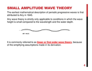
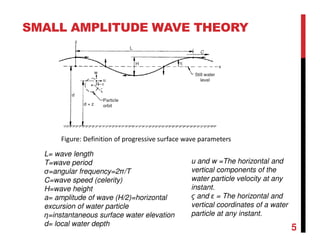
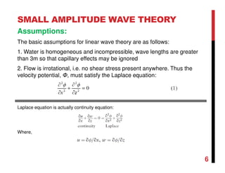
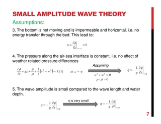
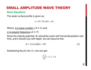
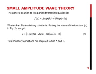
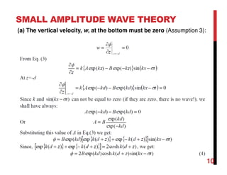
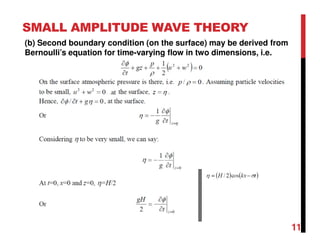
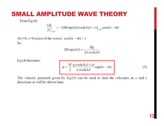
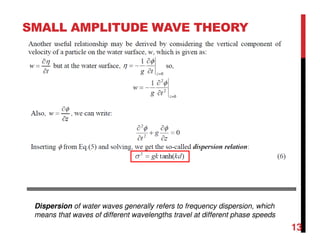
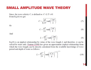
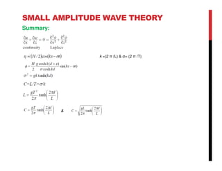
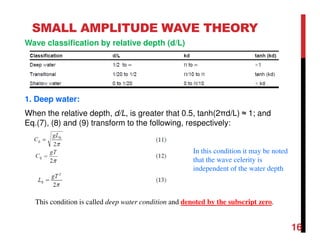
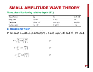
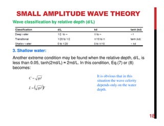
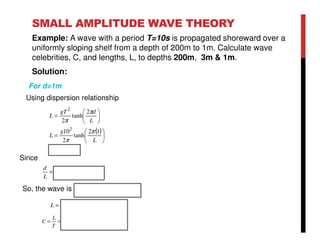
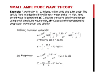
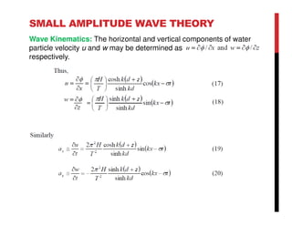
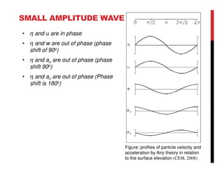
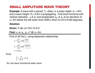
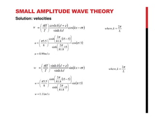
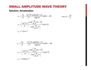
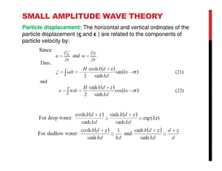
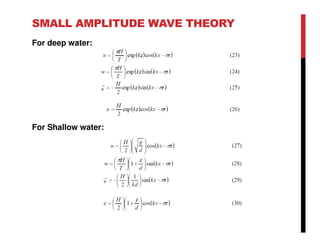
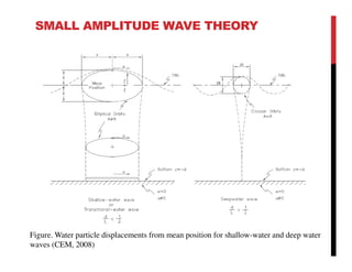
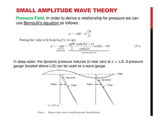
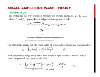
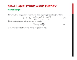
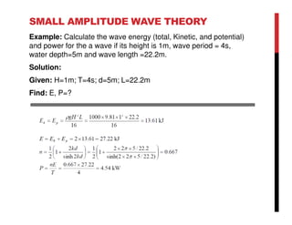
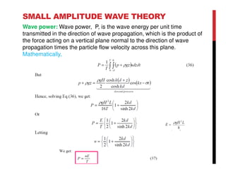
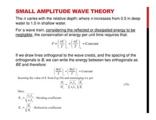
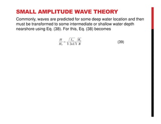
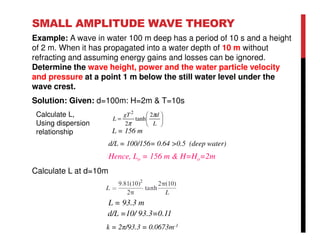
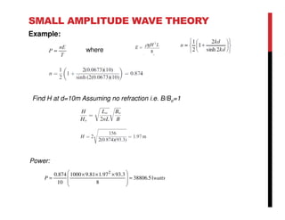
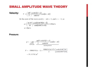
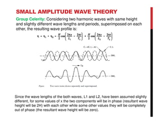
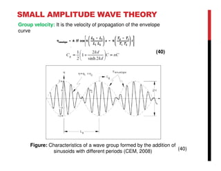
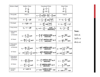
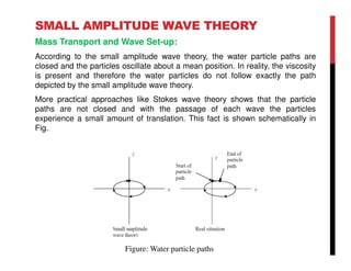
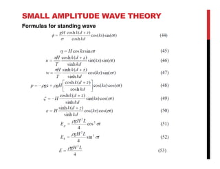
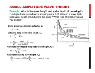
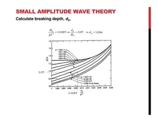
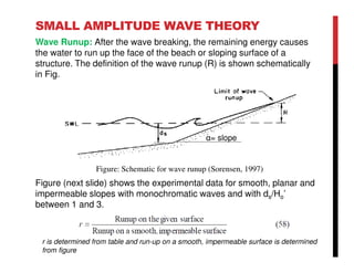
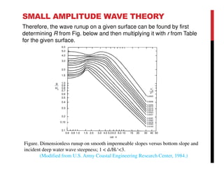
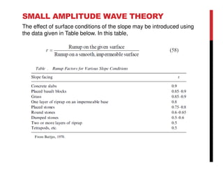
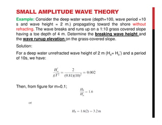
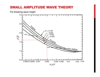
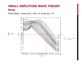
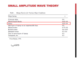
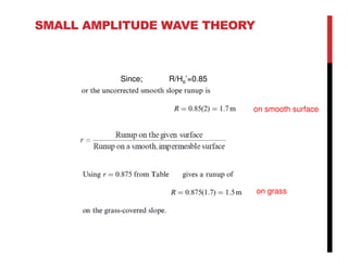
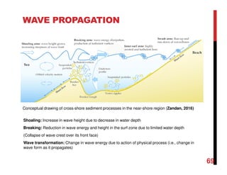


Small amplitude wave theory provides a mathematical description of periodic progressive waves using linear assumptions. It assumes wave amplitude is small compared to wavelength and depth. The key equations derived are the wave dispersion relationship and expressions for water particle velocity, acceleration, and pressure as functions of depth and phase. Wave energy is calculated as the sum of kinetic and potential energy. Wave power is the rate at which wave energy is transmitted shoreward and varies with depth from 0.5 in deep water to 1.0 in shallow water. Wave characteristics like height, length, and celerity change as waves propagate into shallower depths based on conservation of energy.


![Engineering Economics: Solved exam problems [ch1-ch4]](https://cdn.slidesharecdn.com/ss_thumbnails/solvedexamproblemsch1-ch4-200220070043-thumbnail.jpg?width=640&height=640&fit=bounds)