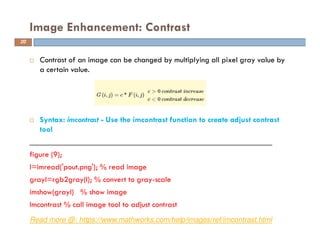
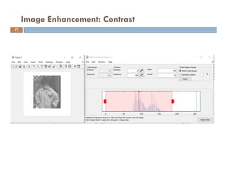
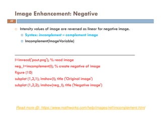
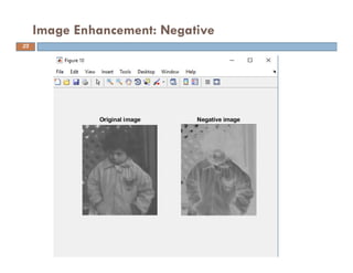
Download as PDF, PPTX
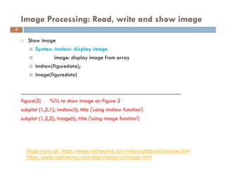
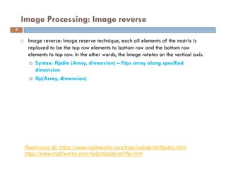
![ Brightness of an image is adjusted with adding or subtracting a certain value
to gray level of each pixel.
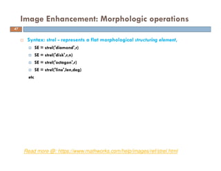
Syntax: imadjust - adjust intensity values or colormap
For gray-scale images
adjusted_image = imadjust(I)
adjusted_image = imadjust(I,[low_in high_in])
For color images
J = imadjust(RGB,[low_in high_in],___)
Image Enhancement: Brightness
Read more @: https://www.mathworks.com/help/images/ref/imadjust.html
15](https://image.slidesharecdn.com/imageprocessingmatlabtutorial-200217154315/85/Basics-of-image-processing-using-MATLAB-15-320.jpg)
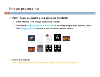
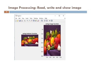
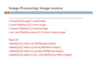
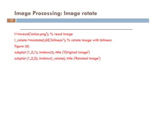
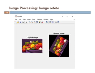
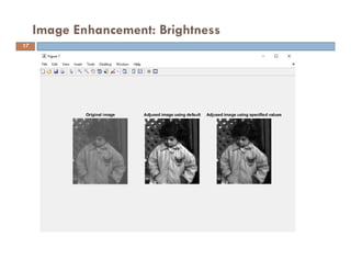
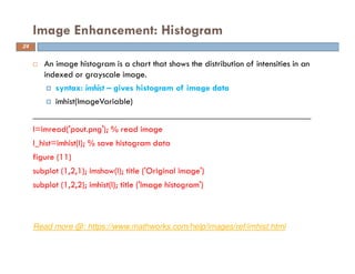
![%Gray-scale image
I=imread(‘pout.png');
grayI=rgb2gray(I);
adj_I= imadjust(grayI); % for gray-scale images
adj_I2=imadjust(grayI,[0.3 0.7],[]); % using specified values
figure (7)
subplot (1,3,1); imshow(grayI); title ('Original image')
subplot (1,3,2); imshow(adj_I); title ('Adjused image using default')
subplot (1,3,3); imshow(adj_I2); title ('Adjused image using specified values')
Image Enhancement: Brightness
16](https://image.slidesharecdn.com/imageprocessingmatlabtutorial-200217154315/85/Basics-of-image-processing-using-MATLAB-16-320.jpg)
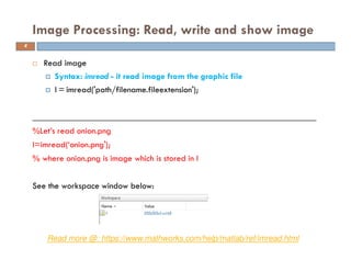
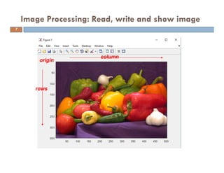
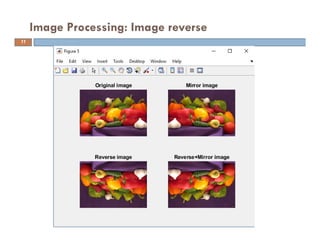
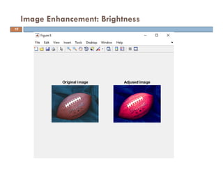
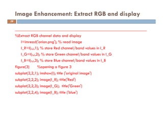
![%Color images
I_RGB = imread(‘football.png');
adj_I_RGB = imadjust(I_RGB, [.2 .3 0; .6 .7 1], []);
figure (8)
subplot (1,2,1); imshow(I_RGB); title ('Original image')
subplot (1,2,2); imshow(adj_I_RGB); title ('Adjused image')
Image enhancement: Brightness
18](https://image.slidesharecdn.com/imageprocessingmatlabtutorial-200217154315/85/Basics-of-image-processing-using-MATLAB-18-320.jpg)
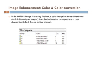
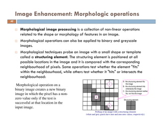
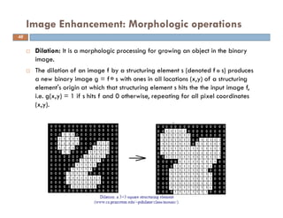

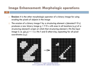

The document provides an overview of image processing techniques using MATLAB, covering command line functions and the image processing toolbox. It includes syntax and examples for reading, displaying, writing images, as well as advanced topics like image manipulation, brightness and contrast adjustments, filtering, and morphological operations. Additionally, the document contains essential references and links to further resources for MATLAB image processing.


![Engineering Economics: Solved exam problems [ch1-ch4]](https://cdn.slidesharecdn.com/ss_thumbnails/solvedexamproblemsch1-ch4-200220070043-thumbnail.jpg?width=640&height=640&fit=bounds)


