Download as PDF, PPTX
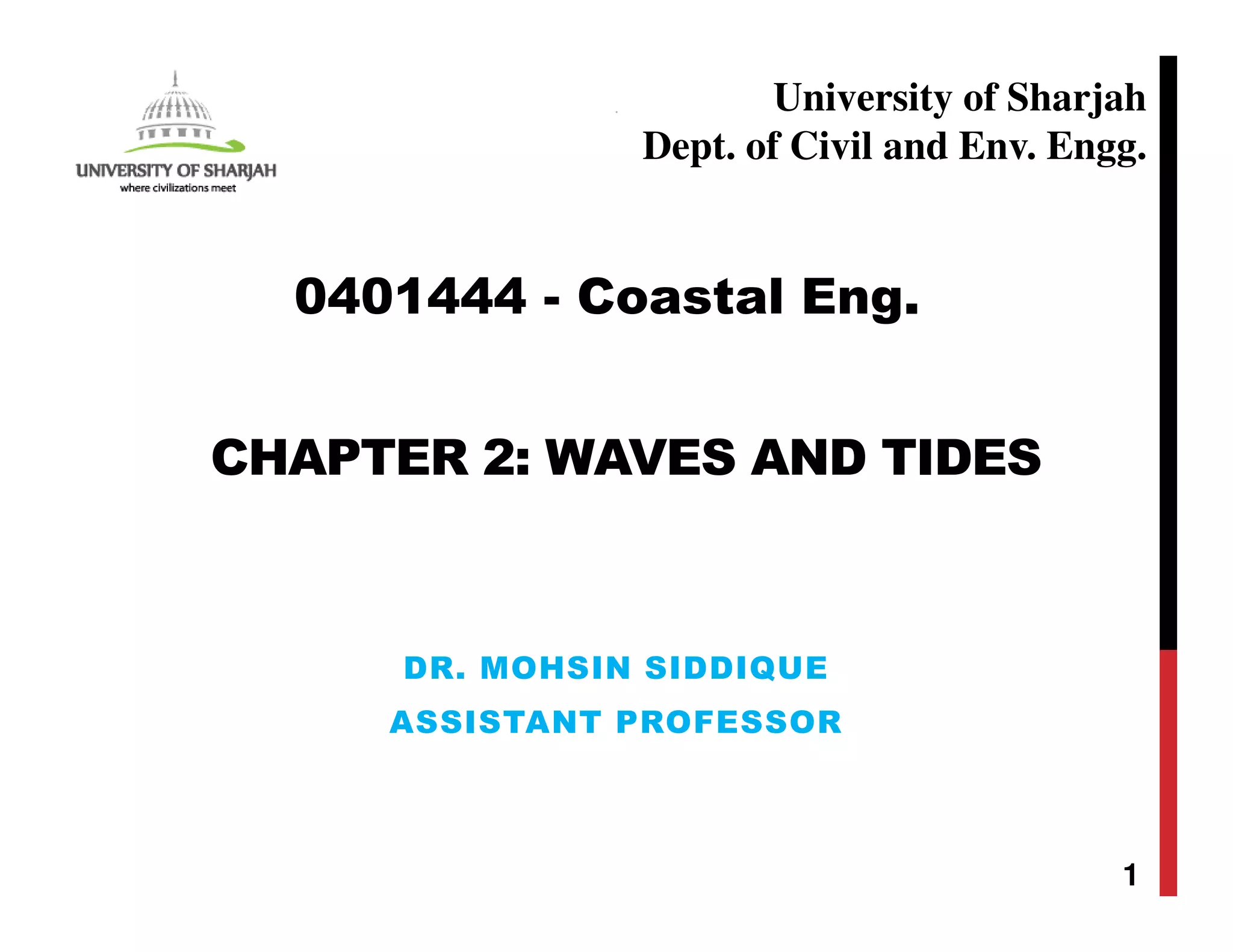


![TSUNAMI: EXAMPLE
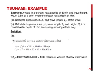
Solution:
(b). To determine the nearshore characteristics, we assume there is
negligible energy dissipation and wave energy in deep and near-shore
are same.
Energy of wave=E=[ρgH2L]/16
L=T (c)
Power of wave=E/T
Eo= Ei
75](https://image.slidesharecdn.com/chapter2waveandtides-180204112927/85/Chapter-2-wave-and-tides-with-examples-75-320.jpg)


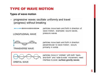
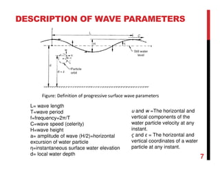
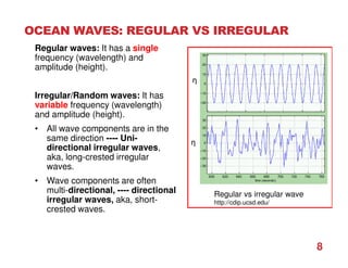
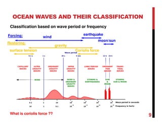
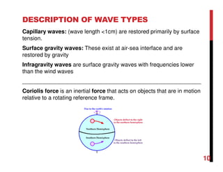
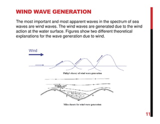
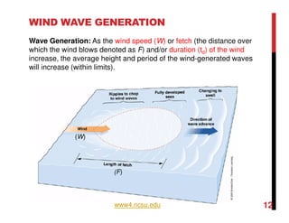
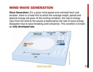
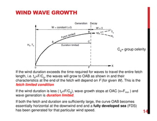
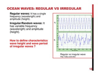
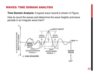
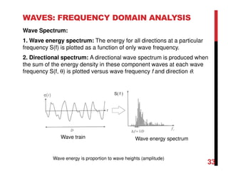
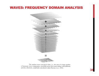
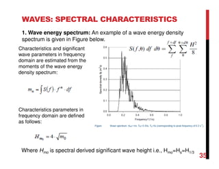
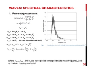
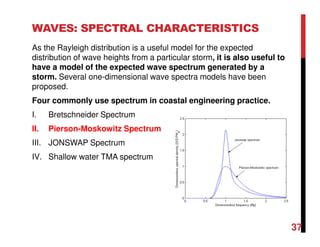
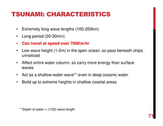
1. Waves are disturbances that transfer energy through a medium, such as water. They can be regular (single frequency/height) or irregular/random (variable frequency/height). 2. Important wave parameters include wavelength, period, frequency, speed, height, amplitude, and water elevation. 3. Ocean waves are classified based on their period/frequency and include capillary, gravity, and infragravity waves. 4. Wind generates waves by transferring energy and momentum to water. Wave characteristics depend on wind speed, fetch (distance over which wind blows), and duration. Fully developed seas occur when energy input balances dissipation.


![Engineering Economics: Solved exam problems [ch1-ch4]](https://cdn.slidesharecdn.com/ss_thumbnails/solvedexamproblemsch1-ch4-200220070043-thumbnail.jpg?width=640&height=640&fit=bounds)