(a) Reynolds number: Re = VL/ (b) Froude number: Fr = V/(gL)1/2

1. River Mechanics
Dimensional Analysis
Dimensional Analysis and
Similarity Laws

2. Reason for Dimensional
Analysis…
 Usually we can’t determine all
essential facts based on theory
alone
 Experiments!
 Erosion Experiment
 We can greatly reduce the
number of tests needed by using
dimensional analysis
 We can derive easier set-ups
using similarity laws!

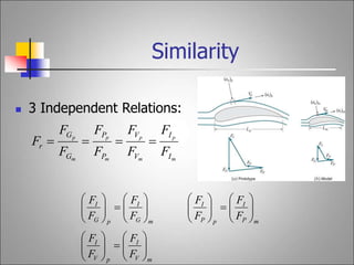
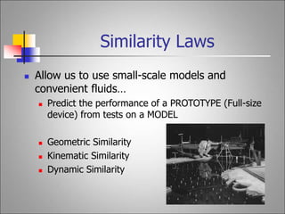
3. Similarity Laws
 Allow us to use small-scale models and
convenient fluids…
 Predict the performance of a PROTOTYPE (Full-size
device) from tests on a MODEL
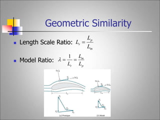
 Geometric Similarity
 Kinematic Similarity
 Dynamic Similarity

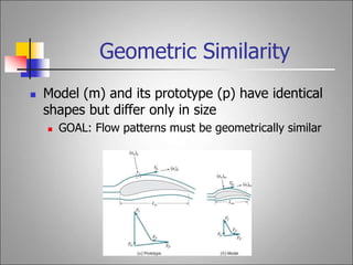
4. Geometric Similarity
 Model (m) and its prototype (p) have identical
shapes but differ only in size
 GOAL: Flow patterns must be geometrically similar

5. Geometric Similarity
m
p
r
L
L
L 
 Length Scale Ratio:
 Model Ratio:
p
m
r L
L
L


1


6. Kinematic Similarity
 IN ADDITION TO GEOMETRIC SIMILARITY,
ratios of velocities at all corresponding points in
flow are same

7. Kinematic Similarity
m
p
r
V
V
V 
 Velocity Scale Ratio:
 Gives rise to Time Scale Ratio:
r
r
r
V
L
T 

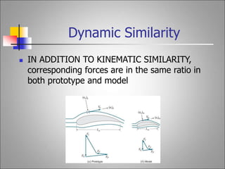
8. Dynamic Similarity
 IN ADDITION TO KINEMATIC SIMILARITY,
corresponding forces are in the same ratio in
both prototype and model

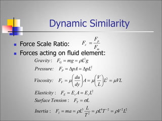
9. Dynamic Similarity
m
p
r
F
F
F 
 Force Scale Ratio:
 Forces acting on fluid element:
2
2
2
4
2
3
2
2
2
3
:
:
:
:
L
V
T
L
T
L
L
ma
F
Inertia
L
F
Tension
Surface
L
E
A
E
F
Elasticity
VL
L
L
V
A
dy
du
F
Viscosity:
pL
pA
F
Pressure:
g
L
mg
F
Gravity
I
T
v
v
E
V
P
G








































10. Similarity
m
p
m
p
m
p
m
p
I
I
V
V
P
P
G
G
r
F
F
F
F
F
F
F
F
F 



 3 Independent Relations:
m
V
I
p
V
I
m
P
I
p
P
I
m
G
I
p
G
I
F
F
F
F
F
F
F
F
F
F
F
F




















































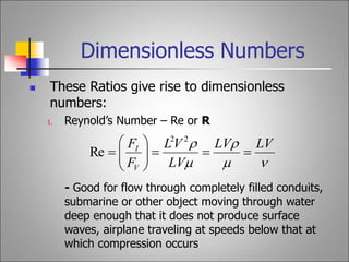
11. Dimensionless Numbers
 These Ratios give rise to dimensionless
numbers:
1. Reynold’s Number – Re or R
- Good for flow through completely filled conduits,
submarine or other object moving through water
deep enough that it does not produce surface
waves, airplane traveling at speeds below that at
which compression occurs




 LV
LV
LV
V
L
F
F
V
I












2
2
Re

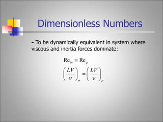
12. Dimensionless Numbers
- To be dynamically equivalent in system where
viscous and inertia forces dominate:
p
m
p
m
LV
LV
















Re
Re

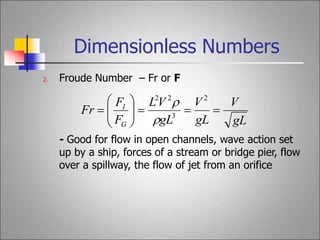
13. Dimensionless Numbers
2. Froude Number – Fr or F
- Good for flow in open channels, wave action set
up by a ship, forces of a stream or bridge pier, flow
over a spillway, the flow of jet from an orifice
gL
V
gL
V
gL
V
L
F
F
Fr
G
I












2
3
2
2



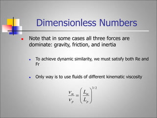
14. Dimensionless Numbers
 Note that in some cases all three forces are
dominate: gravity, friction, and inertia
 To achieve dynamic similarity, we must satisfy both Re and
Fr
 Only way is to use fluids of different kinematic viscosity
2
/
3









p
m
p
m
L
L



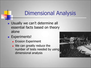
15. Dimensional Analysis
 Usually we can’t determine all
essential facts based on theory
alone
 Experiments!
 Erosion Experiment
 We can greatly reduce the
number of tests needed by using
dimensional analysis

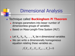
16. Dimensional Analysis
 Technique called Buckingham Pi Theorem
 Arranges parameters into lesser number of
dimensionless groups of variables
 Based on Mass-Length-Time System (MLT)
 Let X1, X2, X3, … , Xn be n dimensional variables
 We can write a dimensionally homogeneous
equation relating these variables as…
  0
,...,
,
,
, 4
3
2
1 
n
X
X
X
X
X
f

17. Dimensional Analysis
 
 
k
n
k
n










,...,
0
,...,
,
2
1
2
1


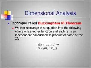
 Technique called Buckingham Pi Theorem
 We can rearrange this equation into the following
where  is another function and each is an
independent dimensionless product of some of the
X’s


18. Dimensional Analysis
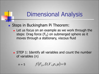
 Steps in Buckingham Pi Theorem:
 Let us focus on an example as we work through the
steps: Drag force (FD) on submerged sphere as it
moves through a stationary, viscous fluid
 STEP 1: Identify all variables and count the number
of variables (n)
n = 5   0
,
,
,
, 


V
D
F
f D

19. Dimensional Analysis
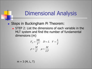
 Steps in Buckingham Pi Theorem:
 STEP 2: List the dimensions of each variable in the
MLT system and find the number of fundamental
dimensions (m)
m = 3 (M, L, T)
LT
M
L
M
T
L
V
L
D
T
ML
FD






 3
2

20. Dimensional Analysis
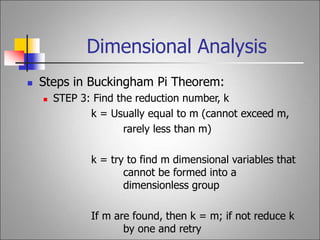
 Steps in Buckingham Pi Theorem:
 STEP 3: Find the reduction number, k
k = Usually equal to m (cannot exceed m,
rarely less than m)
k = try to find m dimensional variables that
cannot be formed into a
dimensionless group
If m are found, then k = m; if not reduce k
by one and retry

21. Dimensional Analysis
 Steps in Buckingham Pi Theorem:
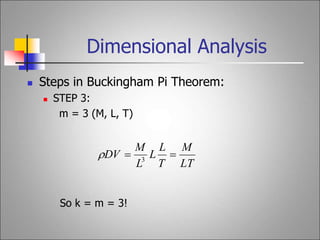
 STEP 3:
m = 3 (M, L, T)
So k = m = 3!
LT
M
T
L
L
L
M
DV 
 3


22. Dimensional Analysis
 Steps in Buckingham Pi Theorem:
 STEP 4: Determine n-k (This is the number of
dimensionless groups needed!)
n-k = 5-3 = 2
 Step 5: Select k variables to be primary (repeating)
variables that contain all m (M, L, T) dimensions
V
D


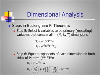
23.  Steps in Buckingham Pi Theorem:
 Step 5: Select k variables to be primary (repeating)
variables that contain all m (M, L, T) dimensions
 Step 6: Equate exponents of each dimension on both
sides of Pi term (M0L0T0):
Dimensional Analysis
D
c
b
a
c
b
a
F
V
D
V
D
2
2
2
2
1
1
1
1







  0
0
0
1
1
1
3
1
1
1
1
1
T
L
M
LT
M
T
L
L
L
M
V
D
c
b
a
c
b
a






















 


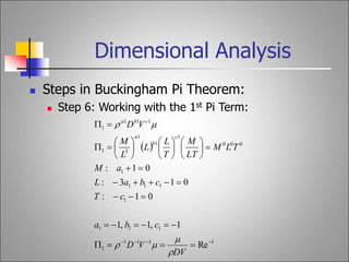
24.  Steps in Buckingham Pi Theorem:
 Step 6: Working with the 1st Pi Term:
Dimensional Analysis
 
1
1
1
1
1
1
1
1
1
1
1
1
1
0
0
0
1
1
1
3
1
1
1
1
1
Re
1
,
1
,
1
0
1
:
0
1
3
:
0
1
:















































DV
V
D
c
b
a
c
T
c
b
a
L
a
M
T
L
M
LT
M
T
L
L
L
M
V
D
c
b
a
c
b
a







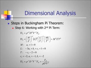
25.  Steps in Buckingham Pi Theorem:
 Step 6: Working with 2nd Pi Term:
Dimensional Analysis
 
2
2
2
2
1
2
1
1
1
1
1
1
1
1
0
0
0
2
1
1
1
3
2
2
2
2
2
2
,
1
,
2
0
2
:
0
1
3
:
0
1
:
V
D
F
F
V
D
b
a
c
c
T
c
b
a
L
a
M
T
L
M
T
ML
T
L
L
L
M
F
V
D
D
D
c
b
a
D
c
b
a

















































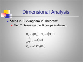
26.  Steps in Buckingham Pi Theorem:
 Step 7: Rearrange the Pi groups as desired:
Dimensional Analysis
   
 
 
Re
Re
2
2
2
2
1
1
2
2
1






V
D
F
V
D
F
D
D










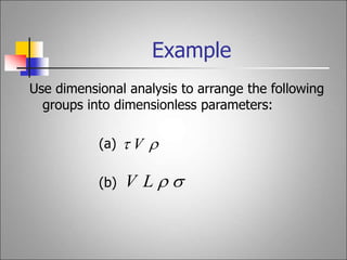
27. Use dimensional analysis to arrange the following
groups into dimensionless parameters:
(a)
(b)
Example

 V


L
V