Geographical Information System (GIS) Georeferencing and Digitization, Bihar Thematic Map making
The document outlines exercises on georeferencing and digitization using a topographical map of Uttar Pradesh and a GIS software (QGIS). It describes the procedures for georeferencing a scanned map, creating point, line, and polygon vector layers, and the importance of ground control points (GCPs) during these processes. Additionally, it explains how to create thematic maps focusing on specific themes like literacy and sex ratio in Bihar using the digitized data.
Introduction to GIS including georeferencing and digitization exercises covering maps and data representation.
Exercises related to georeferencing topographical sheets using QGIS, including step-by-step procedures and GCPs.
Introduction to digitization and creating point layers. The process of setting attributes and managing data layers in GIS.
Guidelines for creating line layers representing linear features such as roads, including layout options.
Instructions for creating polygon layers to mark areas using digitization techniques in GIS.
Exercises on georeferencing and creating layouts for various features in Bihar including railways and district boundaries.
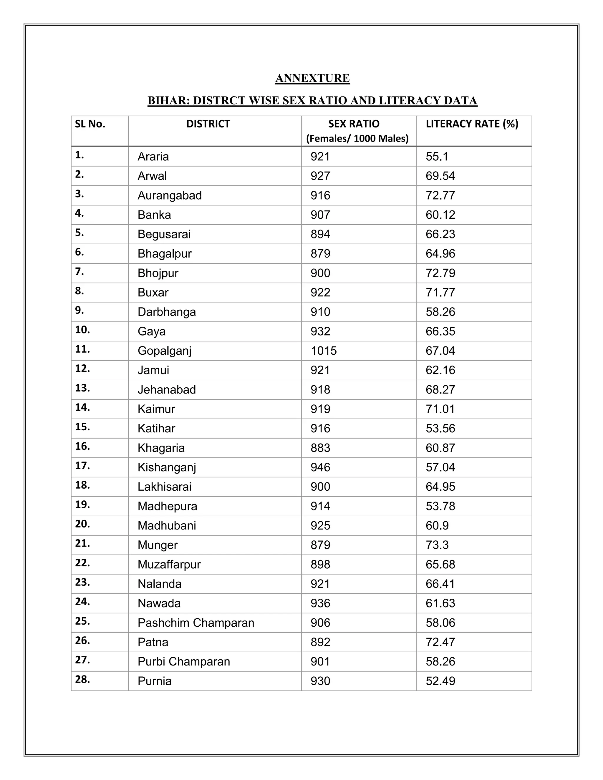
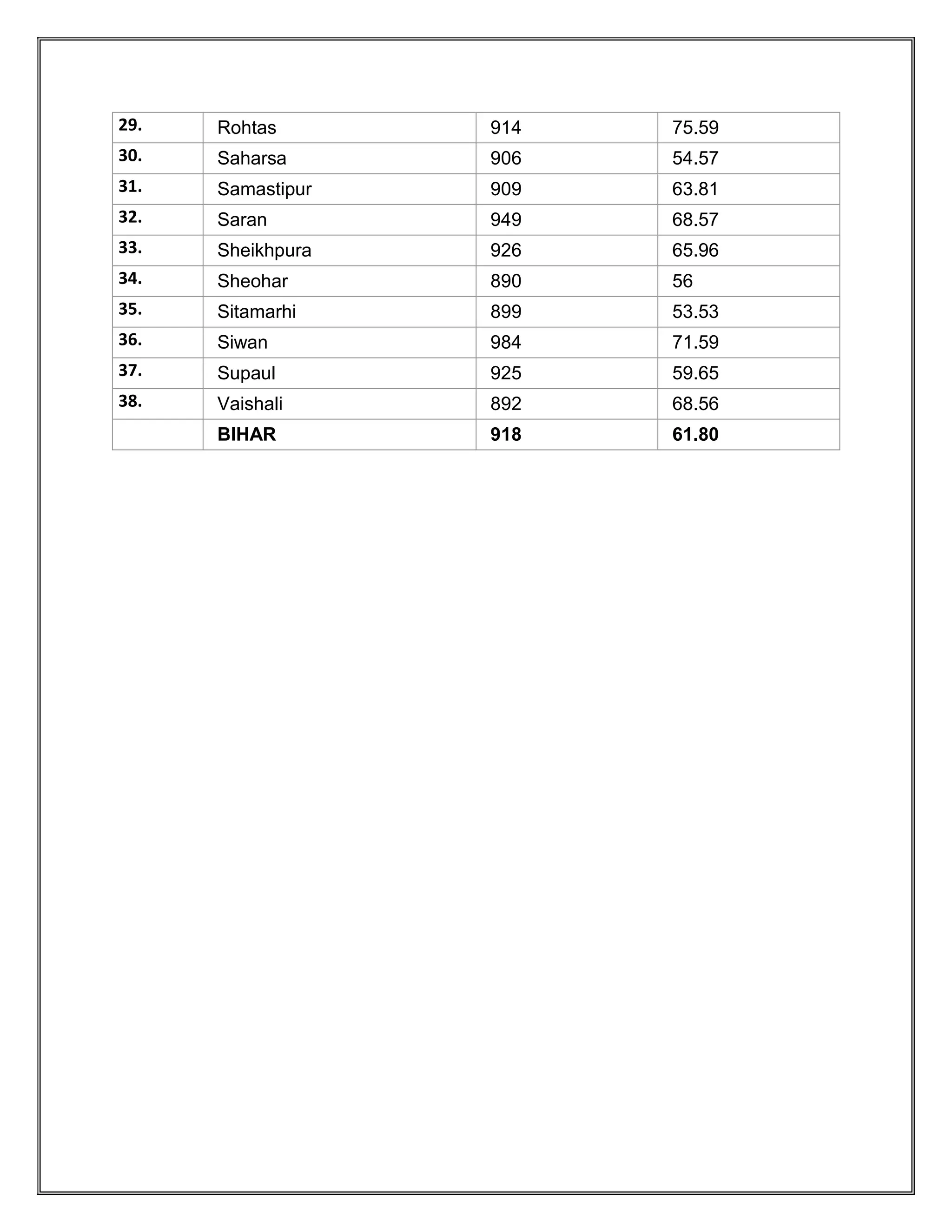
Introduction to thematic maps, procedures for mapping literacy and sex ratio data, and detailed census data for Bihar.District-wise sex ratio and literacy rate data of Bihar, providing specific statistical insights.
CONTENTS
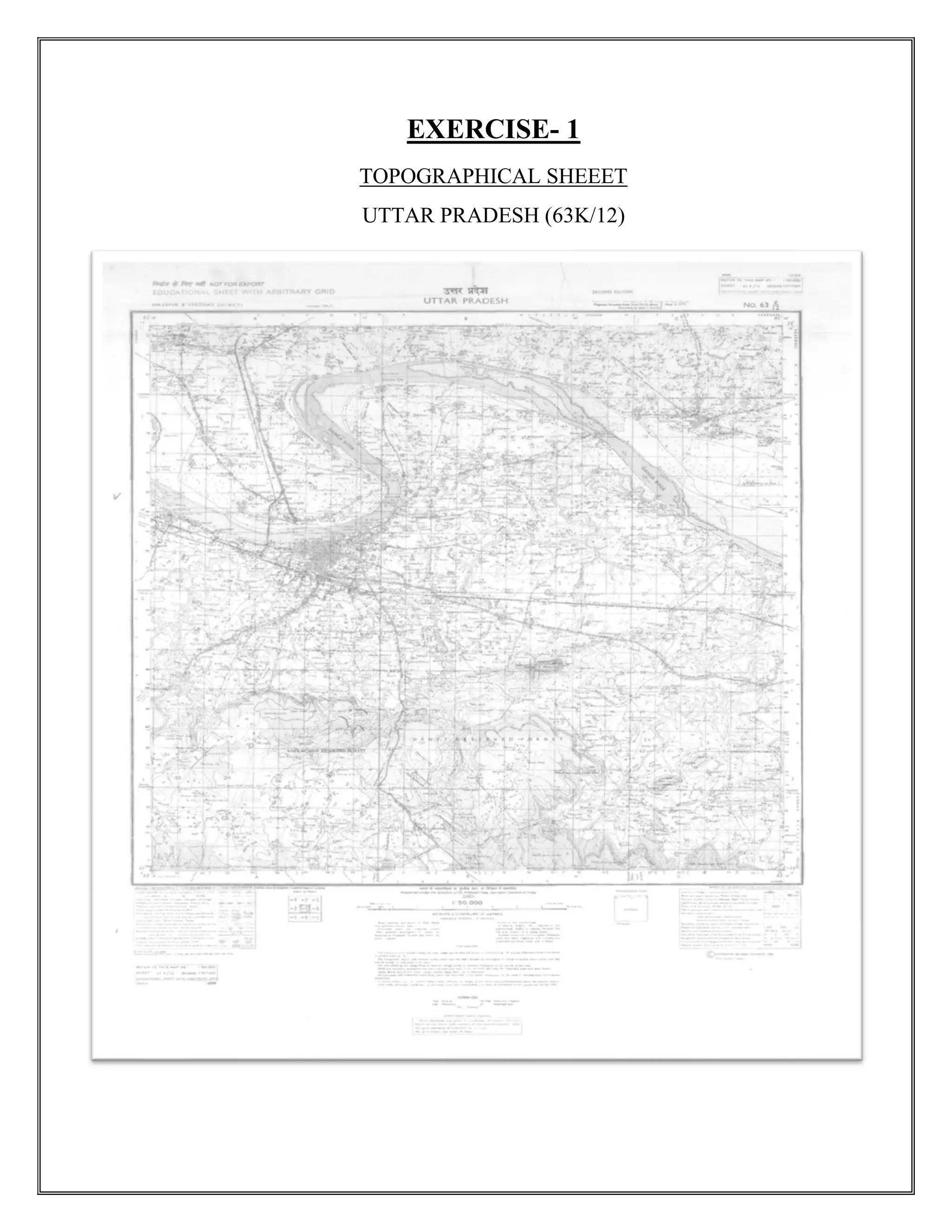
Exercise 1- ScannedImage of the Topographical sheet
Exercise 2- Georeferenced Image of the Topographical sheet
Digitization of Topographical sheet
Exercise 3 - Point
Exercise 4 - Line
Exercise 5 - Area
Bihar Map
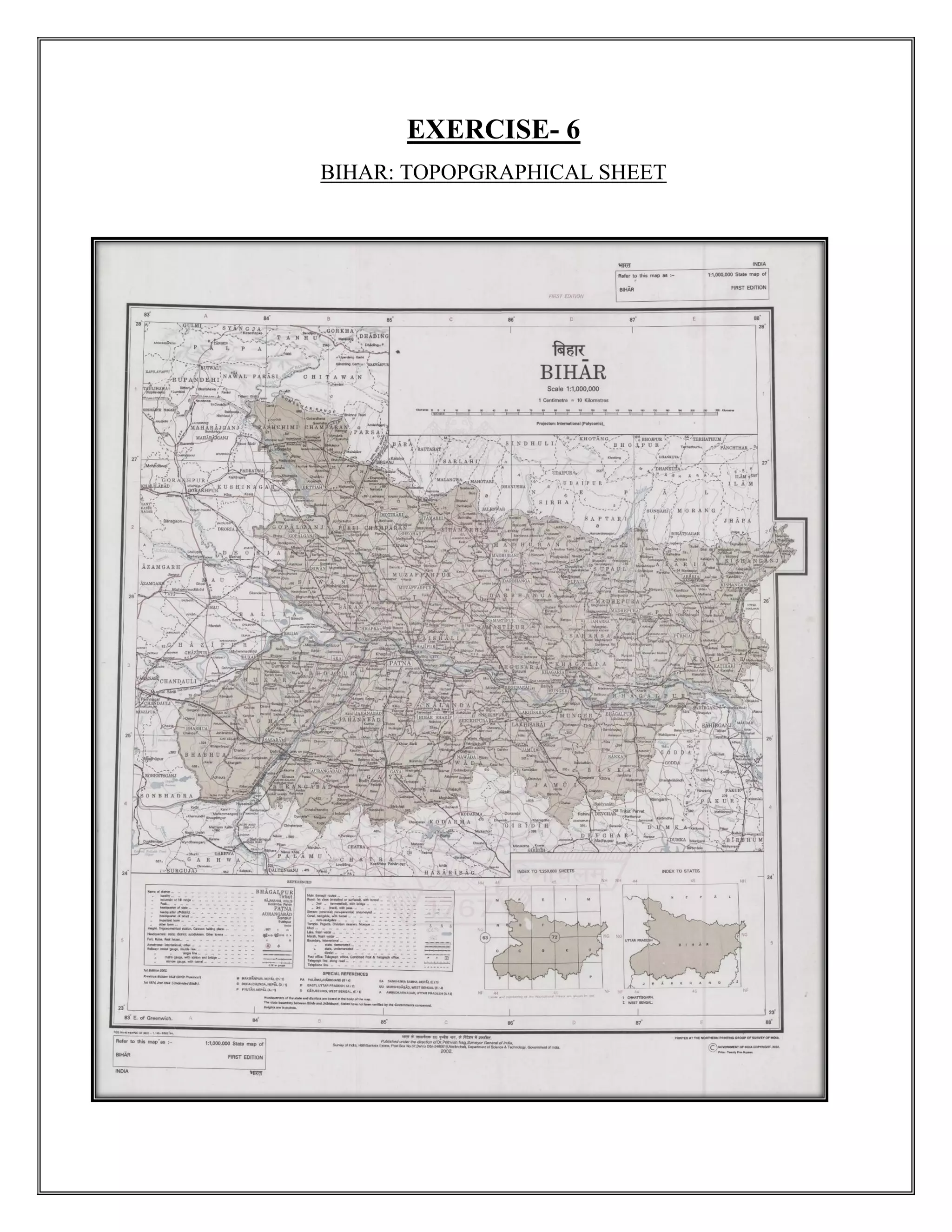
Exercise 6- Scanned Image of the Map
Exercise 7- Georeferenced image of the Map
Digitization of Map
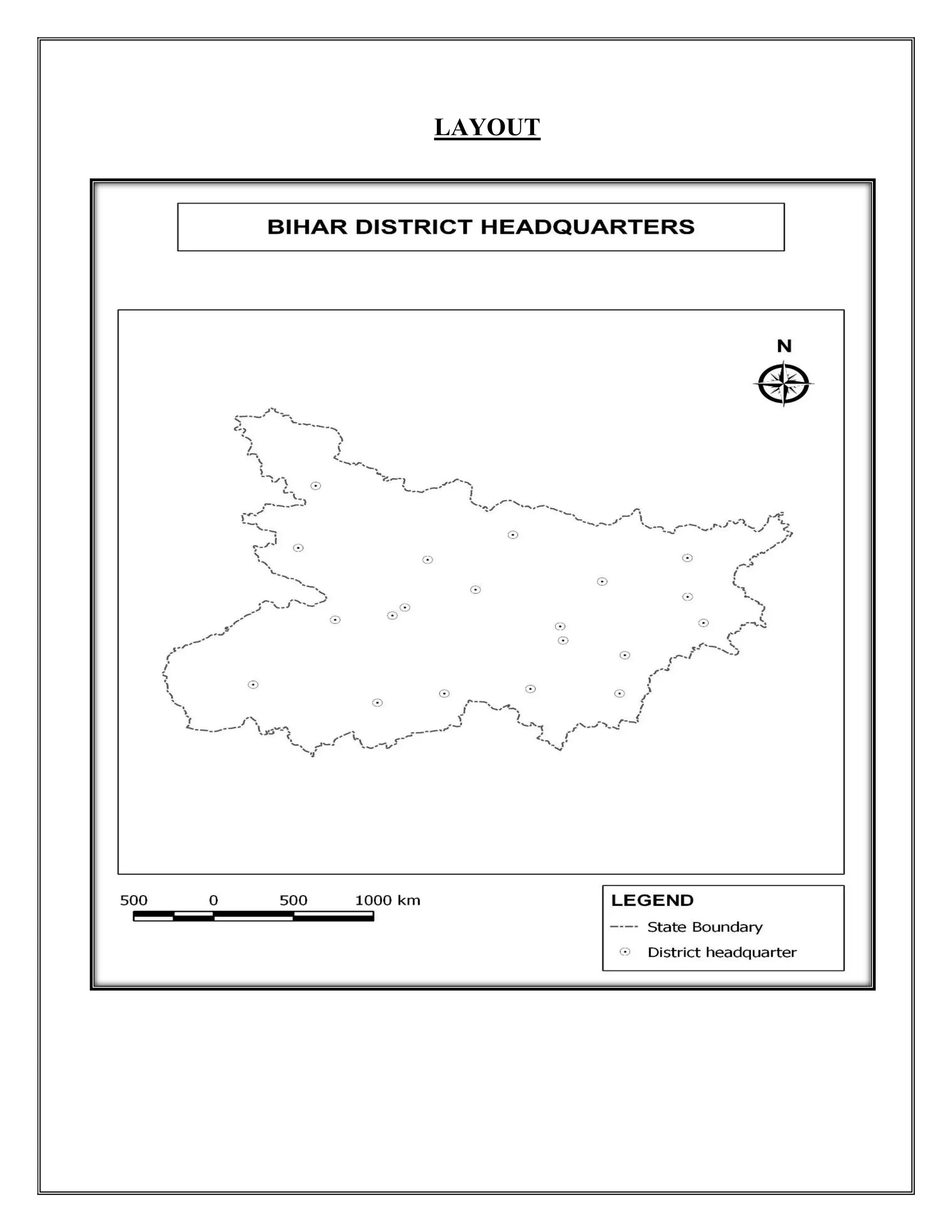
Exercise 8 - District Headquarters
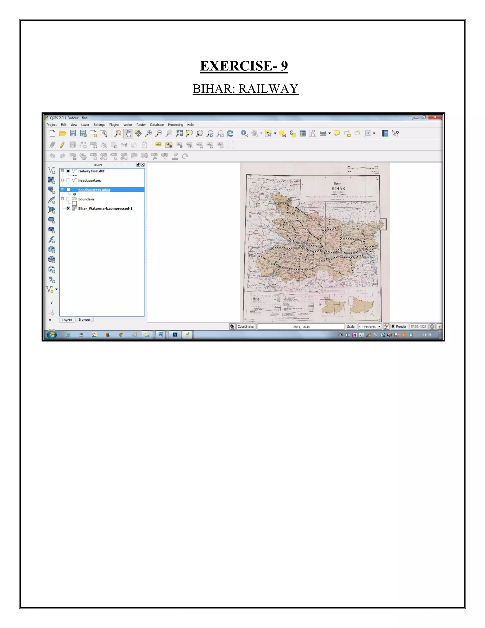
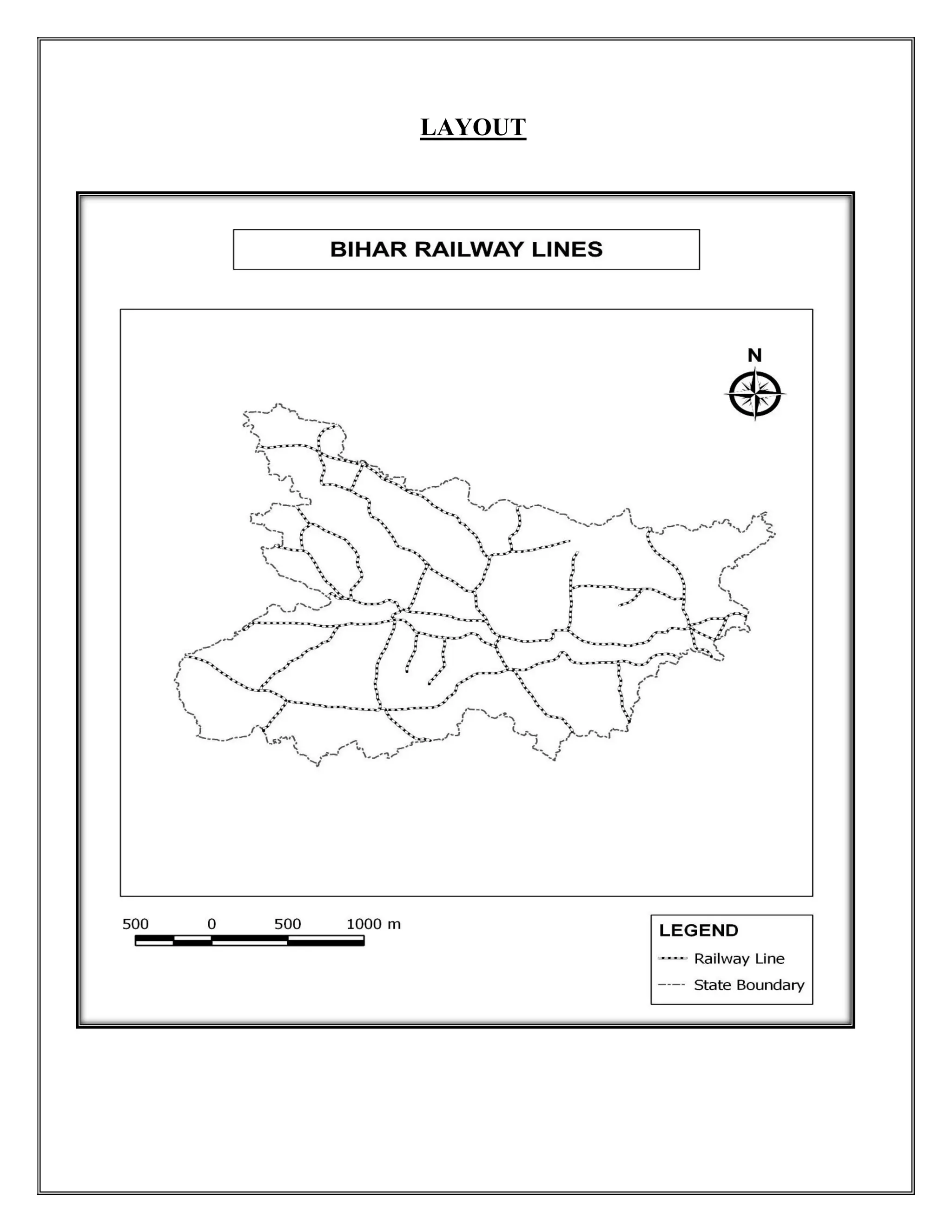
Exercise 9 - Railway of Bihar
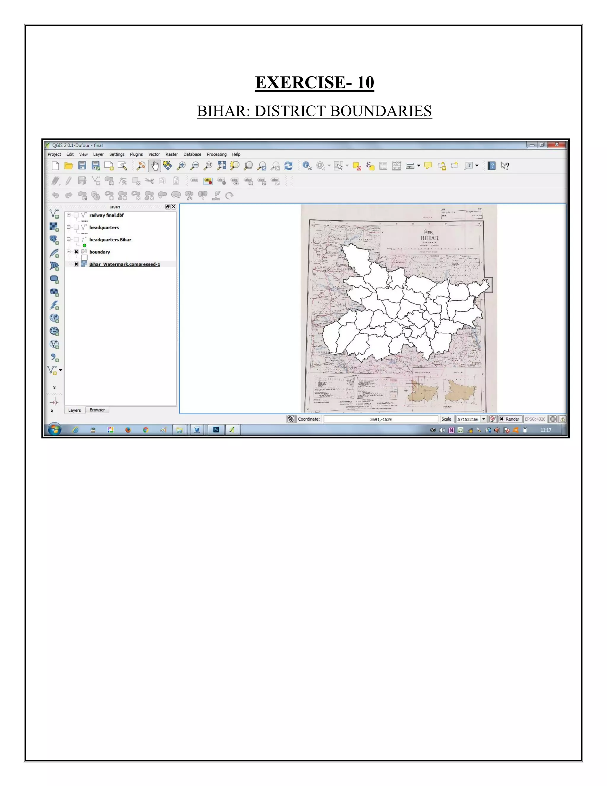
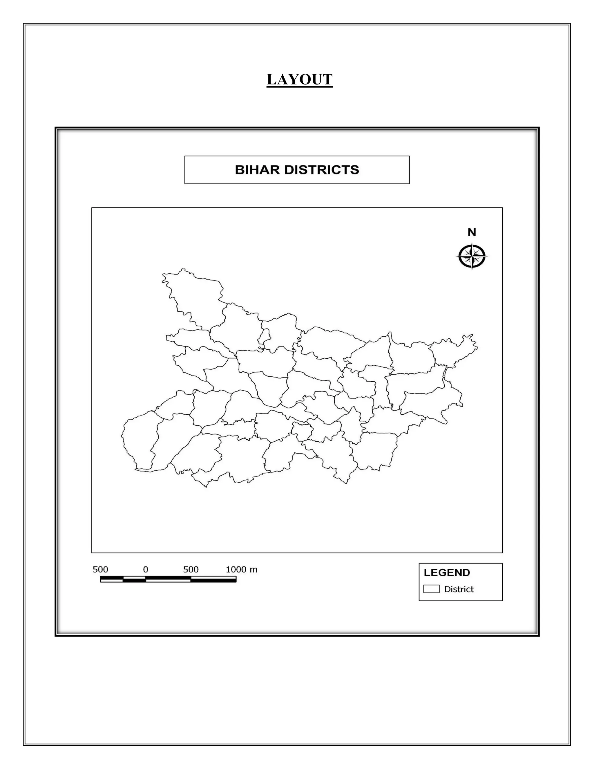
Exercise 10 - District Boundaries
Thematic Maps
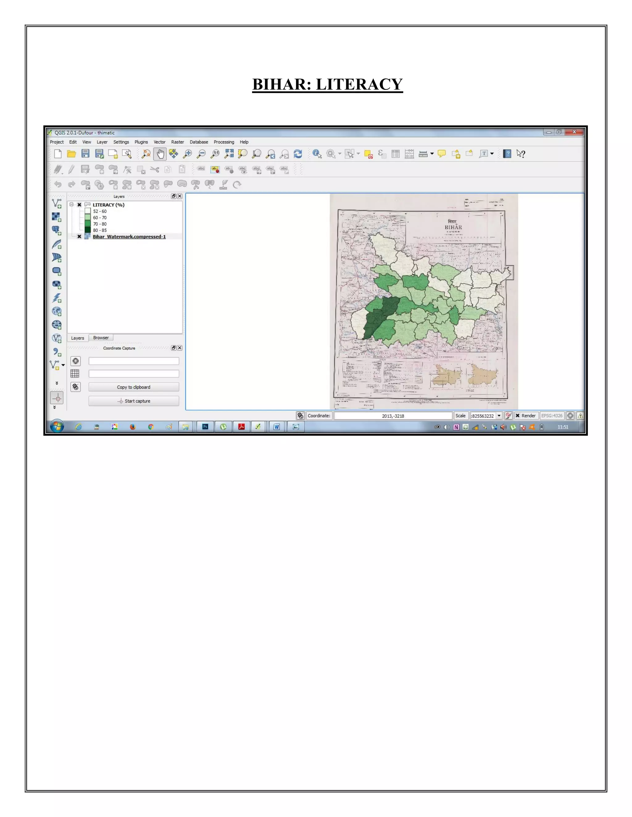
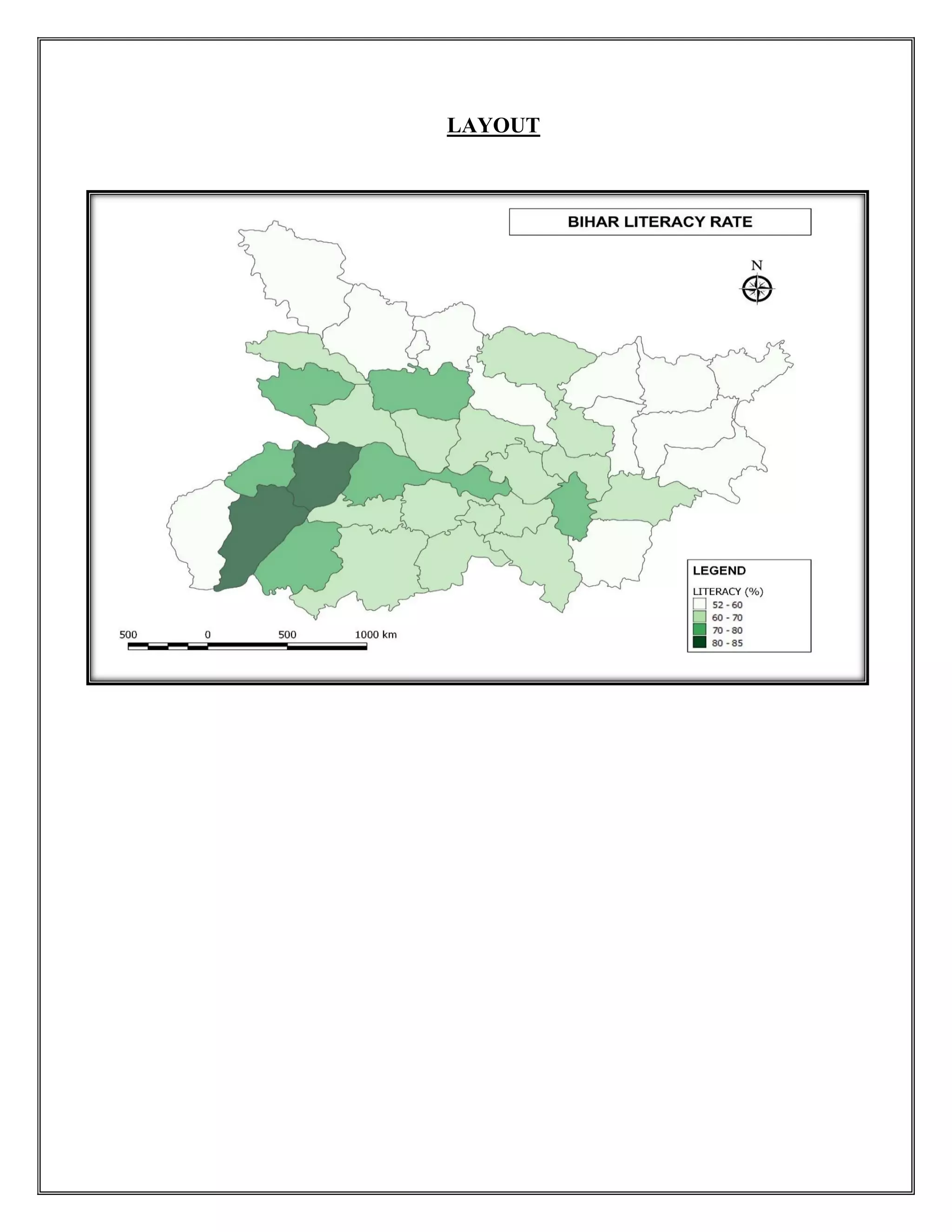
Exercise 11 - Literacy
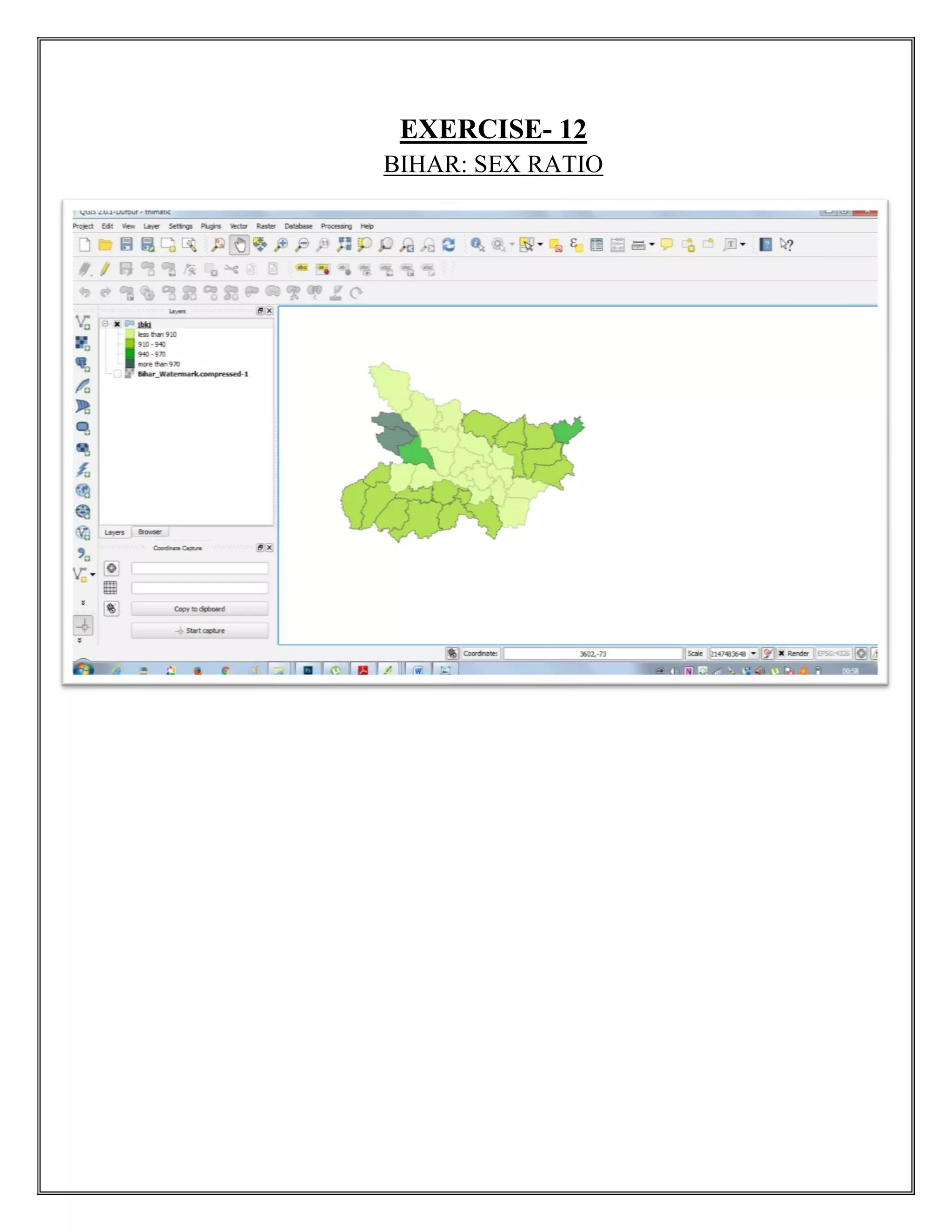
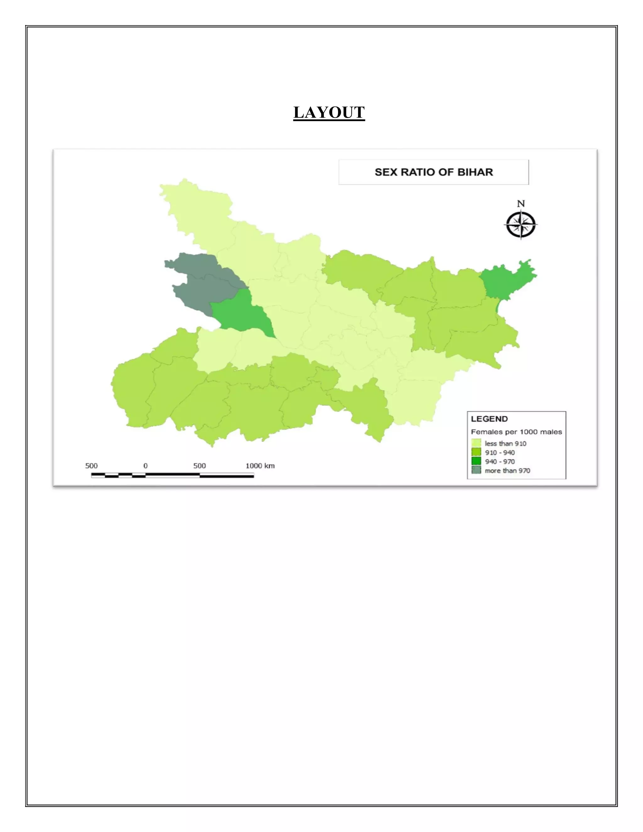
Exercise 12 - Sex Ratio
Annexure
EXERCISE- 2
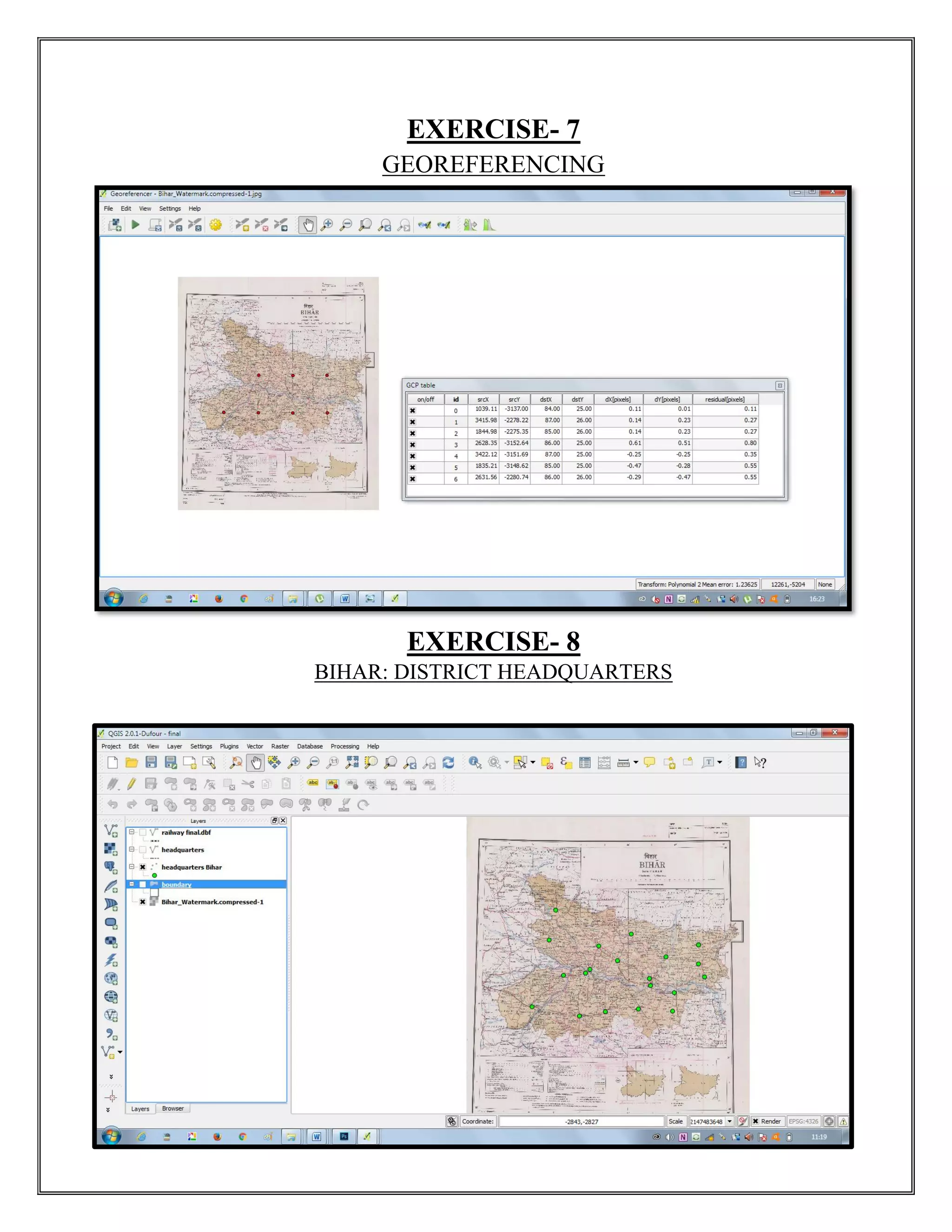
GEOREFERENCING
Introduction
Georeferencing isa process of establishing a mathematical relationship between the image coordinate
system and the real world spatial coordinate system. This mathematical relationship can be assigned by any
one of the transformation settings, viz. Polynomial order 1, 2 or 3, Linear, Projective and Thin Plate Spline
etc. Polynomial order 2 is the most widely used transformation in Georeferencing. Recently Thin Plate
Spline gaining popularity due its ability of incorporating the local deformations in the data, this is very
useful when we are dealing with low resolution data. However, in this practical we are using traditional
polynomial order 2 transformation to perform georeferencing/rectification of the Toposheet.
In this exercise, we will use a topographic Map of Uttar Pradesh. This map is in the Universal Transverse
Mercator(UTM) projection based on WGS 84 Datum.
1. First, we open Quantum GIS (QGIS) via the Start menu. (Start → All Programs → QGIS Dufour →
QGIS Desktop 2.0.1)
2. We then open QGIS Georeferencer via the menu bar. (Raster → Georeferencer → Georeferencer).
3. The Georeferencer is in the form of a window with two parts to it. The upper part is called as 'Main
Work Space' dedicated to display the Raster Map to be georeferenced and it allows the user to input the
geographic or projected coordinates of control points. The lower part, titled 'GCP table', is where the
Ground Control Point data and residuals will be displayed.
4. Add the toposheet to the Georeferencer by clicking on the 'Open Raster' button or from the File menu
(File → Open Raster).
5. You will then be presented with a popup window, navigate to the data folder in which the 'toposheet.tif'
file is kept. Click on the drop-down menu right to the 'File name' and select '[GDAL] GeoTIFF'. Now
select the ‘toposheet.tif’ and click ‘Open’.
6. You will then be presented with the 'Coordinate Reference System Selector' window, from which we
will select the 'WGS 84' under Coordinate reference system of the world section.
7. To georeference an image we use Ground Control Points (GCPs). GCP is a location on the earth's
surface with known coordinates on both earth and Toposheet/ imagery, i.e., geographic and pixel
coordinates respectively. In this we use graticule intersections as GCPs.
8. To start adding GCPs to our map, we first zoom to a corner of the map where we can easily identify the
intersection of the latitude and longitude. Use the scroll wheel of the mouse to zoom in and out of the map.
Use the 'Pan' Button when needed.
9. To add a GCP click on the 'Add point' button, or go via the menu (Edit → Add Point). The mouse will
transform into a '+' sign, which we use to click on the centre of the intersection. Use 'View tool' when
needed.
5.
10. A window'Enter map coordinates' will pop up where we enter the coordinates of the point which we
take from the map. Always enter 'Longitude or Easting' in X field and 'Latitude or Northing' in Y field. Use
'space bar' in the key board to separate the Degree value from Minutes value and then click ‘OK’.
11. In this exercise we are using the 'Polynomial 2' transformation to georeference the image. For the
'Polynomial 2' transformation we will require minimum 6+1(for check) i.e., 7 GCPs or more GCPs on the
map. Therefore, we need to mark at least 7 GCPs. The GCPs locations should be spread out as much as
possible and they should not be co-linear at the same time they should enclose our whole area. Use the
above procedure to mark six more control points.
12. We now set the spatial reference settings for the toposheet by clicking on the 'Transformation Settings'
button. The 'Transformation Settings' window pops up in which we will enter the spatial information of our
map.
13. Click on the 'Transformation type' drop-down menu and select 'Polynomial 2'. This means we will be
using a second order polynomial transformation.
14. Click on the button next to ‘Output Raster'. A dialogue box will appear in which we enter the name of
our output file. It is recommended to include the name of the original file in this file for example
'Toposheet_WGS84_georef.tif ', This helps us to keep track of our work.
15. ‘Check’ the check box 'Load in QGIS when done' and 'Use 0 for transparency when needed', leave the
reset of the values as default and click 'OK'.
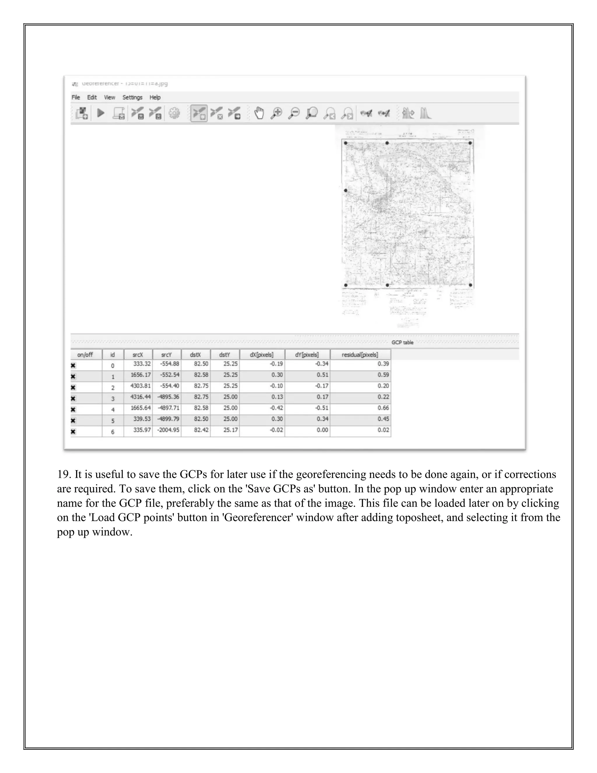
16. After Click 'OK', the last column 'residual [pixels]' displays some values. These are the error values
associated with the GCPs. An error value of 1 or less would be satisfactory.
17. Double check and adjust the GCP locations if the value is greater than 1. To adjust a point, click on the
'Move GCP Point' button, and then click and drag the point to the desired location. Use 'Delete Point'
button to delete an erroneous GCP. We can also enable and disable the GCPs by using check boxes under
'on/off' column in 'GCP Table'.
18. Once the error is around or below 1, click the 'Start Georeferencing' Button. The processing will take at
about 2 minutes. The georeferenced image will be found at the location specified for the 'Output File' in
step 15. You can also notice, the output file loaded in QGIS canvas.
6.
19. It isuseful to save the GCPs for later use if the georeferencing needs to be done again, or if corrections
are required. To save them, click on the 'Save GCPs as' button. In the pop up window enter an appropriate
name for the GCP file, preferably the same as that of the image. This file can be loaded later on by clicking
on the 'Load GCP points' button in 'Georeferencer' window after adding toposheet, and selecting it from the
pop up window.
7.
DIGITIZATION
Introduction
Digitization is theprocess of converting analog data into digital data sets. In GIS context
digitization refers to creating vector datasets viz., point, line or polygon from raster datasets. It is a
way of tracing/recording geographic features in vector format from georeferenced images or maps.
With the help of digitization, we can create different set of layers Viz. Rivers, roads, schools, ward
boundaries and building blocks from a single map; this process is known as Vectorization. Vector
data is easy to edit, update and is more accurate as compared to raster data. Vector data is more
efficient for GIS analysis. Due to these reasons Vectorization is the first step in many GIS projects.
However, it is a time-consuming process and needs a lot of attention to prevent introduction of
errors in the datasets. Vector data is mainly of three types
- Point: It consists of single points having (X, Y) coordinates, for example lamp posts, bus stops
and postbox positions etc.
- Line: It consists a series of (X, Y) coordinates in a sequence (from start node to end node with a
number of vertices joining these two nodes). For example, roads, power lines, ward boundaries and
contours etc.
- Polygon: It is a series of (X, Y) coordinates in a sequence closing a figure where first and last
points are the same. For example, lakes, building blocks, village blocks, ward areas and forests etc.
In this exercise we will use the output of ‘IGET_GIS_003: Georeferencing a Toposheet tutorial’ as
our input.
Open the raster layer of georeferenced toposheet of IGET_GIS_003 tutorial in the map canvas
of Quantum GIS via, ‘Main menu bar → Layer → Add Raster Layer’ or else directly click on icon
from the toolbar → browse and select the georeferenced raster layer in tutorial data → Click on
‘Open’ in the popup window.
8.
EXERCISE- 3
Point LayerCreation
1.To create new point layer, go to main menu bar in QGIS interface and select ‘Layer’! ‘New’!
‘New Shapefile Layer’.
2. Now the ‘New vector Layer’ window will popup. Select ‘Type’ as ‘Point’ as we are interested in
creating a point layer.
3. Specify CRS same as original layer, i.e., as ‘EPSG:4326 - WGS 84’. To do this click on
‘Specify CRS’! Select the ‘WGS 84’ under Coordinate reference system of the world! Click on
‘OK’
4. We can add new required attribute fields to the vector layer that we have created. For example,
if we are creating point vector layer of all temples we can add ‘Name’ of the temple as new field
and ‘intake capacity’, ‘Address’ etc. as other fields.
5. For Each New attribute added, an appropriate name, type of the variable (like text, whole
number, decimal number and date) and width must be selected. Click on ‘Add to attribute List’ and
the attribute will be added to the list.
6. Once the required attributes are added, click on ‘OK’.
7. Now you will be presented with ‘Save As’ window, save the file in appropriate drive with
appropriate name for example: temple up.shp. Once the layer is saved it opens as point data layer
under map legend.
8. To start digitization, we have to enable the editing mode of the corresponding vector layer.
Right click on temple up.shp’ point layer and click on ‘Toggle Editing’
9.You will notice a pencil symbol on left side of the layer name. This tells you that the layer is
ready for editing.
10. Zoom into the toposheet where temples are present, the symbol of hospital in the given
toposheet is. Click on Add feature icon from digitizing toolbar.
11. Place the pointer at the center of the feature of interest and click.
12.You will be presented with an ‘Attributes’ window. Fill the required attribute information like
‘id’, ‘Name’ and ‘Intake_Cap’ (Intake Capacity), ‘Address’. Click ‘OK’.
9.
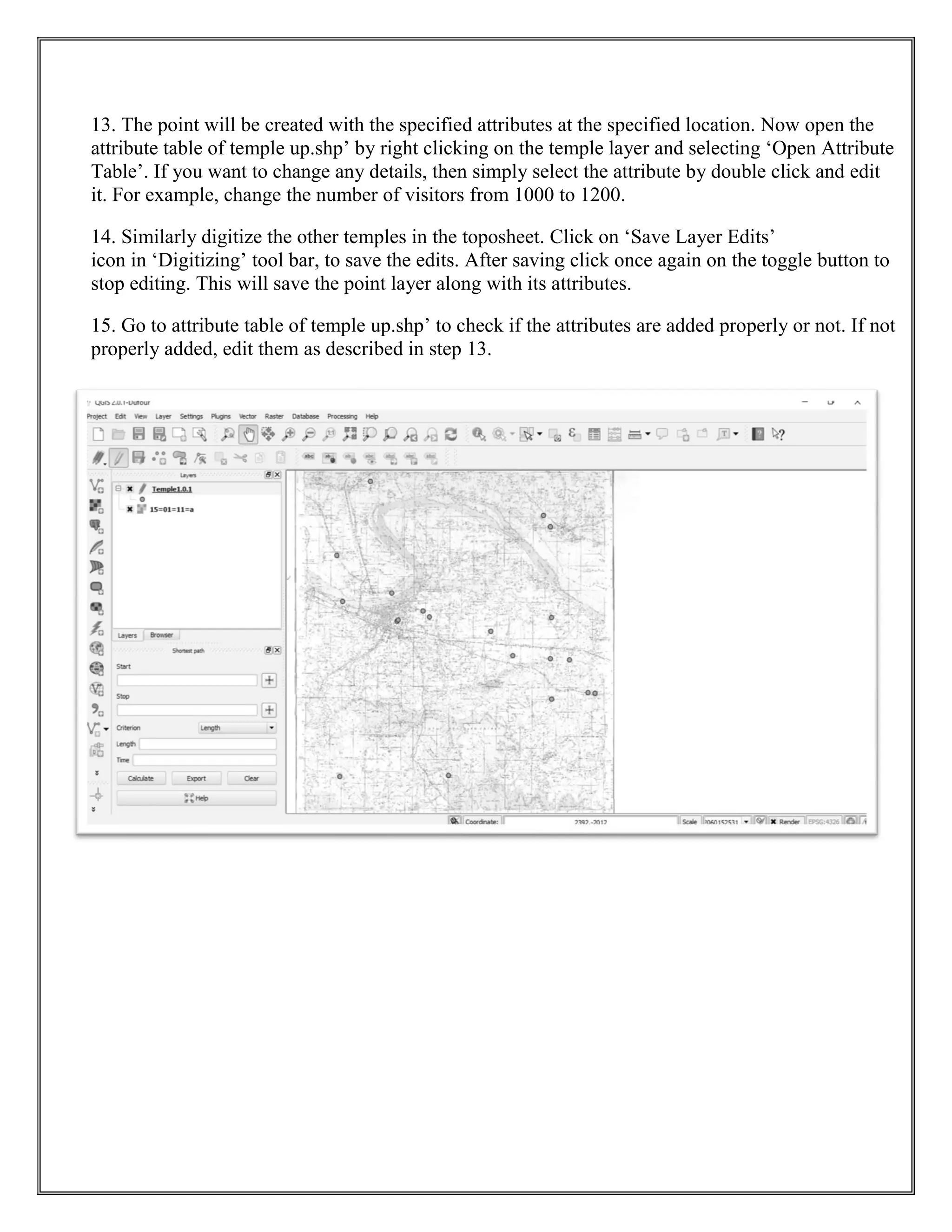
13. The pointwill be created with the specified attributes at the specified location. Now open the
attribute table of temple up.shp’ by right clicking on the temple layer and selecting ‘Open Attribute
Table’. If you want to change any details, then simply select the attribute by double click and edit
it. For example, change the number of visitors from 1000 to 1200.
14. Similarly digitize the other temples in the toposheet. Click on ‘Save Layer Edits’
icon in ‘Digitizing’ tool bar, to save the edits. After saving click once again on the toggle button to
stop editing. This will save the point layer along with its attributes.
15. Go to attribute table of temple up.shp’ to check if the attributes are added properly or not. If not
properly added, edit them as described in step 13.
10.
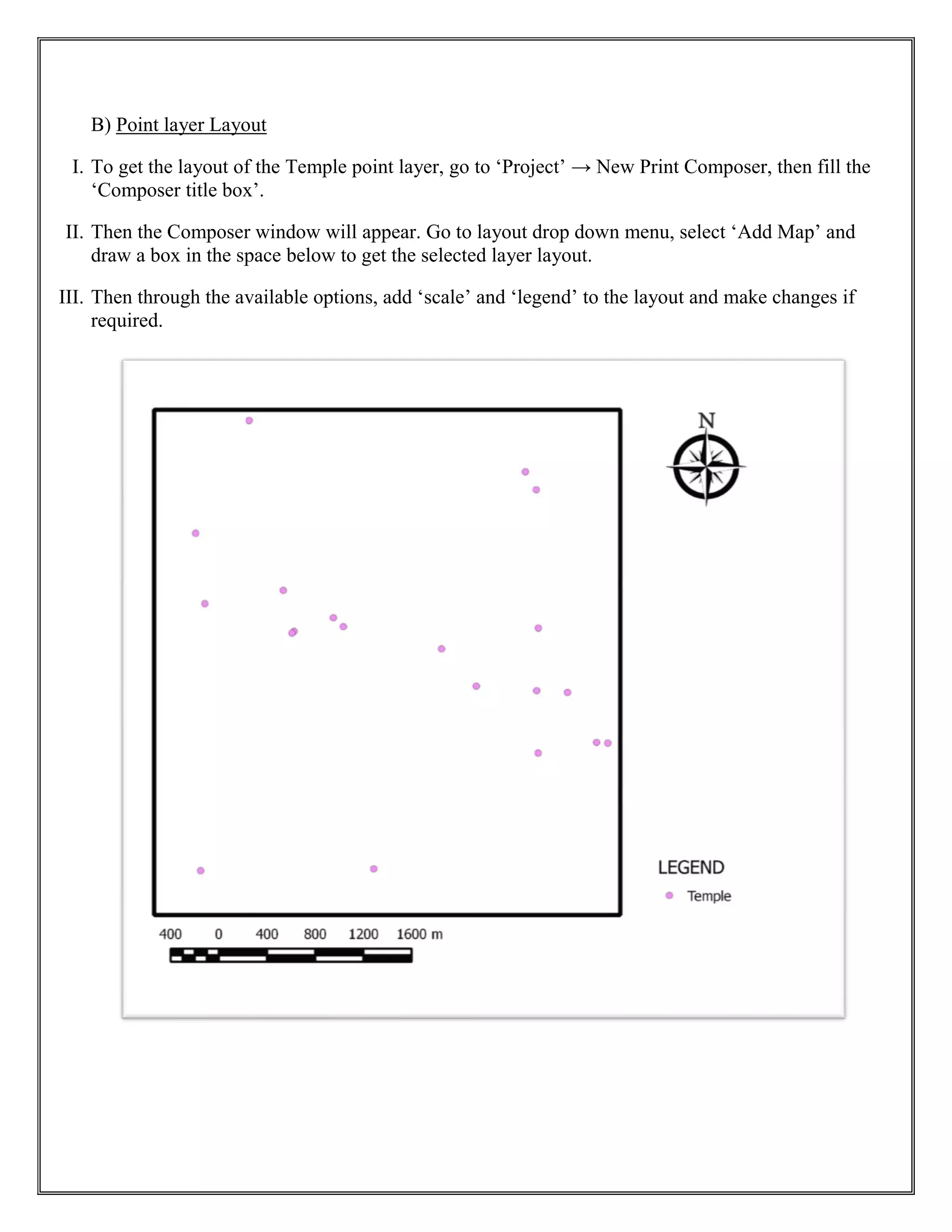
B) Point layerLayout
I. To get the layout of the Temple point layer, go to ‘Project’ → New Print Composer, then fill the
‘Composer title box’.
II. Then the Composer window will appear. Go to layout drop down menu, select ‘Add Map’ and
draw a box in the space below to get the selected layer layout.
III. Then through the available options, add ‘scale’ and ‘legend’ to the layout and make changes if
required.
11.
EXERCISE- 4
Line Layercreation:
A) Line is basically used to represent any linear network such as road, railways and drainage etc.
1. To create line layer, go to ‘Layer’ ! ‘New’ ! ‘New Shapefile Layer’. The ‘New vector Layer’
window will open up. Select ‘Type’ as ‘Line’ as we are interested in creating Line layer of roads
and Specify CRS as ‘EPSG: 4326 – WGS 84’.
2. Add required attributes, for example ‘Name’ as shown in above figure and click ‘OK’. ‘Save
As’ window will open up. Browse to an appropriate location and give an appropriate name for
example ‘Drainage-UP’ ! click on ‘Save’.
3. The layer is created and will be listed in Map legend. Right click on layer, click on ‘Toggle
Editing’ or click on icon from ‘Digitizing’ toolbar.
4. Zoom into the toposheet where river are seen. Click on ‘Add feature’ icon from ‘Digitizing’
toolbar.
5. Now trace cursor along the middle of the road by using left mouse button to insert vertices when
you think the road changes its profile, this means you have to insert more vertices while digitizing
bends to get smooth curve. When you reach a junction or at the end of the road click on the right
mouse button to stop. Now ‘Attributes’ window will open, fill in the appropriate attributes for
example Name is ‘Left bank Yamuna’ and click ‘OK’.
6. Snapping tolerance can be set manually. Go to ‘Settings’ ! ‘snapping Options’.
7. Check the box to the left side of river layer and set ‘Mode’ to ‘vertex and segment’. Specify
tolerance as ‘5’ pixels. Check on ‘Enable topological editing’. And click ‘OK’
8. So by use of the snapping tool it is possible to get an accurate intersection of roads. Once you
finish digitizing all roads in the toposheet save the edits and stop editing by clicking on ‘Toggle
editing’ button. Now the road network along with its attributes will be saved.
12.
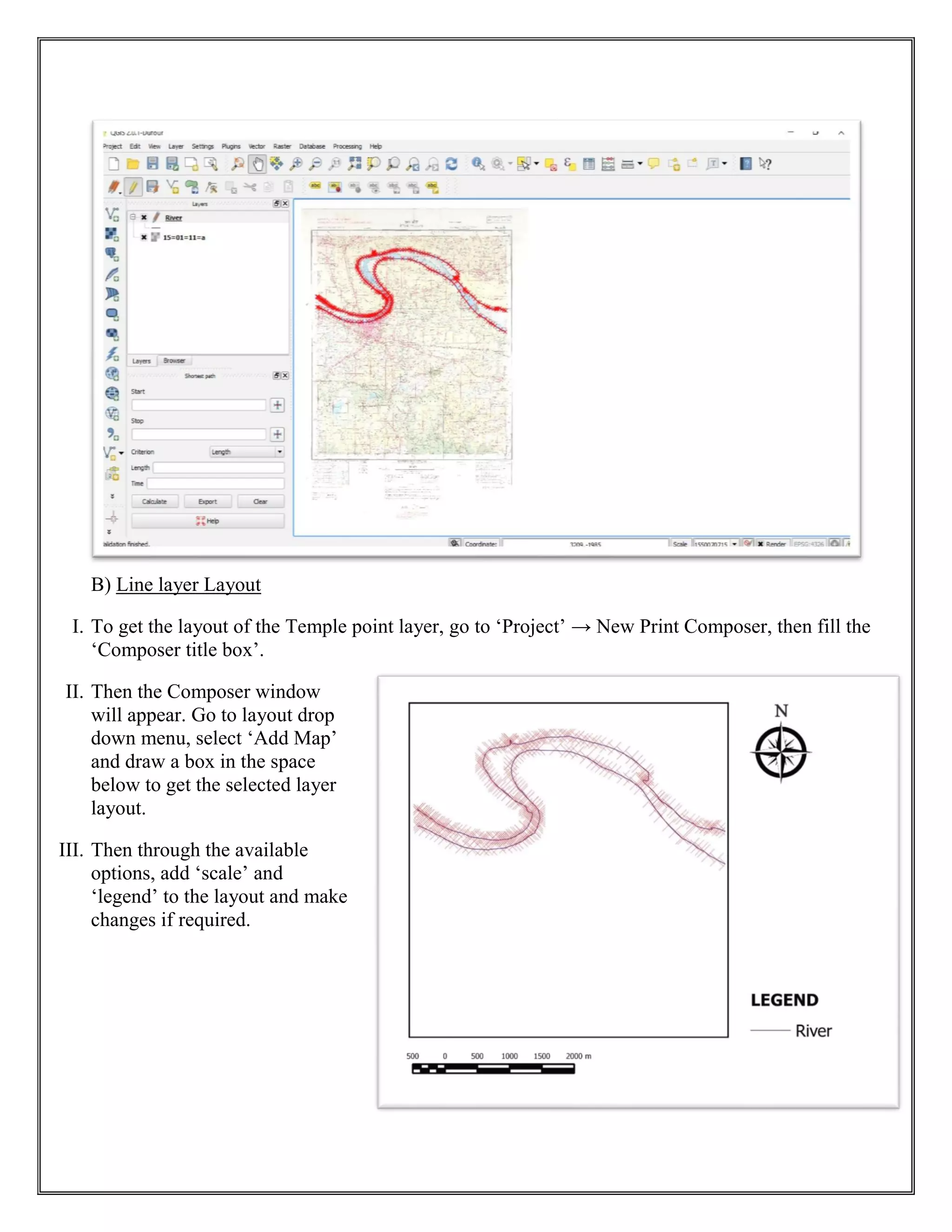
B) Line layerLayout
I. To get the layout of the Temple point layer, go to ‘Project’ → New Print Composer, then fill the
‘Composer title box’.
II. Then the Composer window
will appear. Go to layout drop
down menu, select ‘Add Map’
and draw a box in the space
below to get the selected layer
layout.
III. Then through the available
options, add ‘scale’ and
‘legend’ to the layout and make
changes if required.
13.
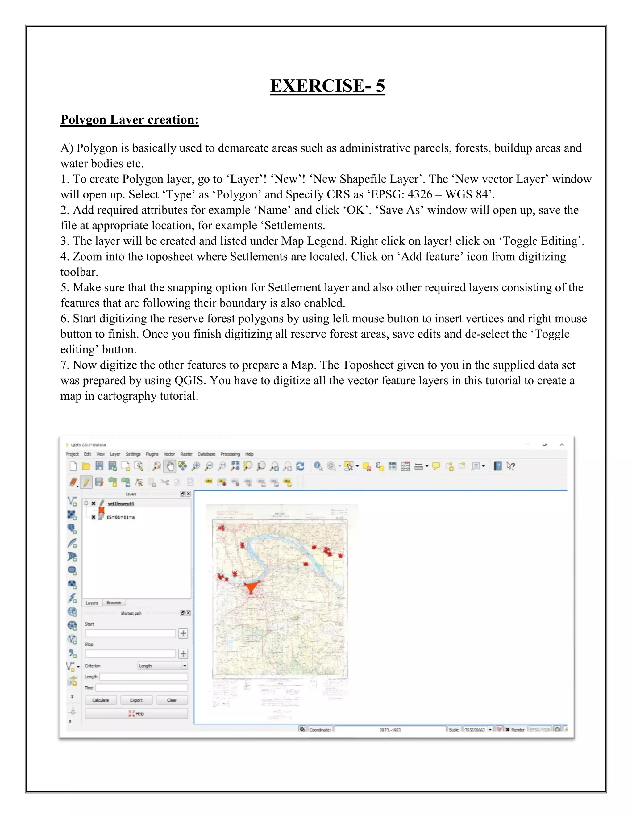
EXERCISE- 5
Polygon Layercreation:
A) Polygon is basically used to demarcate areas such as administrative parcels, forests, buildup areas and
water bodies etc.
1. To create Polygon layer, go to ‘Layer’! ‘New’! ‘New Shapefile Layer’. The ‘New vector Layer’ window
will open up. Select ‘Type’ as ‘Polygon’ and Specify CRS as ‘EPSG: 4326 – WGS 84’.
2. Add required attributes for example ‘Name’ and click ‘OK’. ‘Save As’ window will open up, save the
file at appropriate location, for example ‘Settlements.
3. The layer will be created and listed under Map Legend. Right click on layer! click on ‘Toggle Editing’.
4. Zoom into the toposheet where Settlements are located. Click on ‘Add feature’ icon from digitizing
toolbar.
5. Make sure that the snapping option for Settlement layer and also other required layers consisting of the
features that are following their boundary is also enabled.
6. Start digitizing the reserve forest polygons by using left mouse button to insert vertices and right mouse
button to finish. Once you finish digitizing all reserve forest areas, save edits and de-select the ‘Toggle
editing’ button.
7. Now digitize the other features to prepare a Map. The Toposheet given to you in the supplied data set
was prepared by using QGIS. You have to digitize all the vector feature layers in this tutorial to create a
map in cartography tutorial.
14.
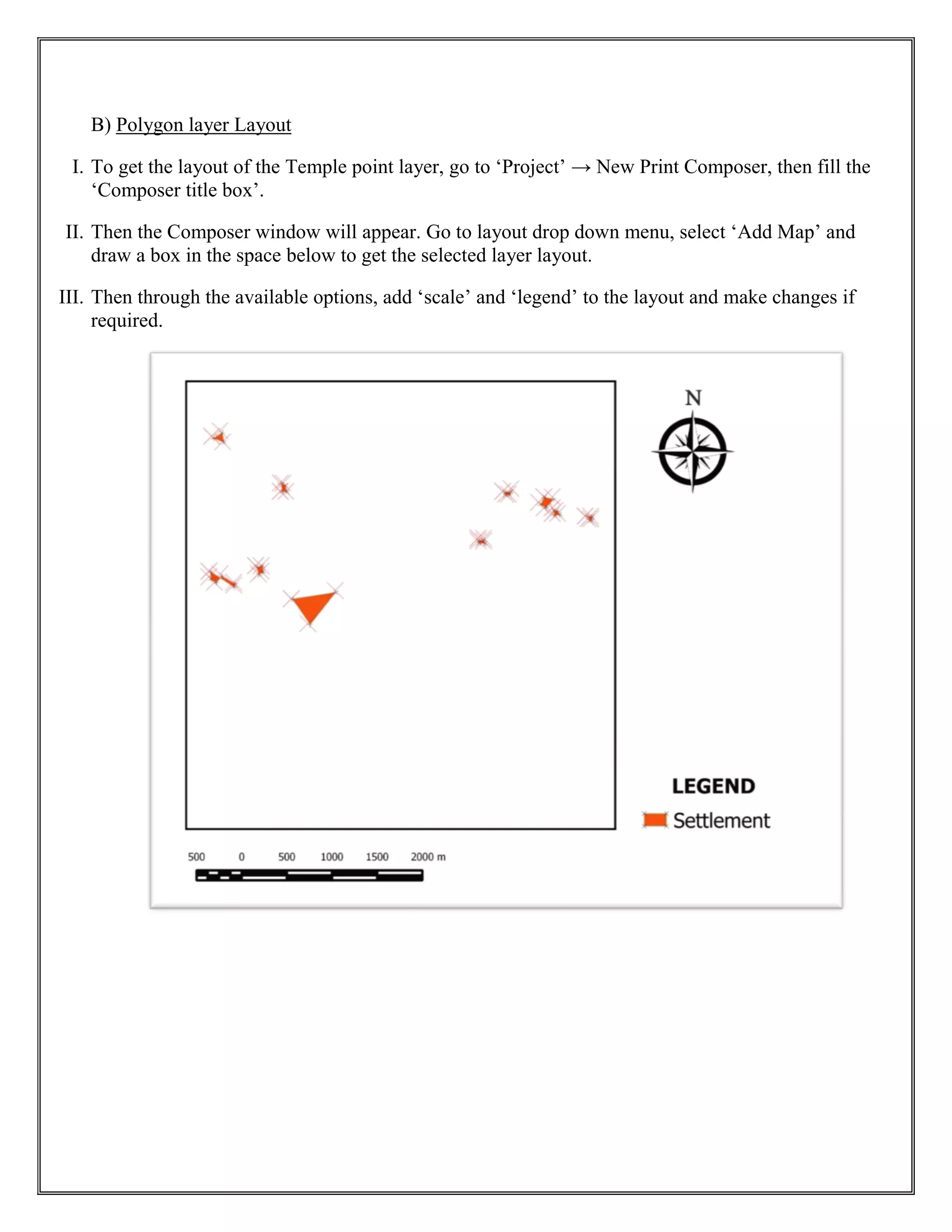
B) Polygon layerLayout
I. To get the layout of the Temple point layer, go to ‘Project’ → New Print Composer, then fill the
‘Composer title box’.
II. Then the Composer window will appear. Go to layout drop down menu, select ‘Add Map’ and
draw a box in the space below to get the selected layer layout.
III. Then through the available options, add ‘scale’ and ‘legend’ to the layout and make changes if
required.
THEMATIC MAP
Introduction
A Thematicmap is a map that emphasizes a particular theme or special topic such as the sex
ratio, literacy rate in an area. They are different from general reference maps because they
do not just show natural features like rivers, cities, political subdivisions and highways.
Instead, if these items are on a thematic map, they are simply used as reference points to
enhance one’s understanding of the map's theme and purpose. They provide specific
information about particular locations and spatial patterns.
In this exercise, we made thematic map of Bihar showing sex ratio and literacy rate with the
help of digitization.
Procedure
1. We took the data for literacy and sex ratio of each district of Bihar from the 2011 census.
This data was divided into 4 class intervals.
2. Then, separate layers were created for each interval using polygon feature and districts
falling in each of these class intervals were marked.
3. Next a separate shade was assigned to each category starting from dense shade for those
having highest value to lighter shade showing districts having lower value.
4. Once digitization of all layers is done, the layer edits were saved and the Toggle editing
button was deselected.
![EXERCISE- 2
GEOREFERENCING
Introduction
Georeferencing is a process of establishing a mathematical relationship between the image coordinate
system and the real world spatial coordinate system. This mathematical relationship can be assigned by any
one of the transformation settings, viz. Polynomial order 1, 2 or 3, Linear, Projective and Thin Plate Spline
etc. Polynomial order 2 is the most widely used transformation in Georeferencing. Recently Thin Plate
Spline gaining popularity due its ability of incorporating the local deformations in the data, this is very
useful when we are dealing with low resolution data. However, in this practical we are using traditional
polynomial order 2 transformation to perform georeferencing/rectification of the Toposheet.
In this exercise, we will use a topographic Map of Uttar Pradesh. This map is in the Universal Transverse
Mercator(UTM) projection based on WGS 84 Datum.
1. First, we open Quantum GIS (QGIS) via the Start menu. (Start → All Programs → QGIS Dufour →
QGIS Desktop 2.0.1)
2. We then open QGIS Georeferencer via the menu bar. (Raster → Georeferencer → Georeferencer).
3. The Georeferencer is in the form of a window with two parts to it. The upper part is called as 'Main
Work Space' dedicated to display the Raster Map to be georeferenced and it allows the user to input the
geographic or projected coordinates of control points. The lower part, titled 'GCP table', is where the
Ground Control Point data and residuals will be displayed.
4. Add the toposheet to the Georeferencer by clicking on the 'Open Raster' button or from the File menu
(File → Open Raster).
5. You will then be presented with a popup window, navigate to the data folder in which the 'toposheet.tif'
file is kept. Click on the drop-down menu right to the 'File name' and select '[GDAL] GeoTIFF'. Now
select the ‘toposheet.tif’ and click ‘Open’.
6. You will then be presented with the 'Coordinate Reference System Selector' window, from which we
will select the 'WGS 84' under Coordinate reference system of the world section.
7. To georeference an image we use Ground Control Points (GCPs). GCP is a location on the earth's
surface with known coordinates on both earth and Toposheet/ imagery, i.e., geographic and pixel
coordinates respectively. In this we use graticule intersections as GCPs.
8. To start adding GCPs to our map, we first zoom to a corner of the map where we can easily identify the
intersection of the latitude and longitude. Use the scroll wheel of the mouse to zoom in and out of the map.
Use the 'Pan' Button when needed.
9. To add a GCP click on the 'Add point' button, or go via the menu (Edit → Add Point). The mouse will
transform into a '+' sign, which we use to click on the centre of the intersection. Use 'View tool' when
needed.](https://image.slidesharecdn.com/gis-180330192010/75/Geographical-Information-System-GIS-Georeferencing-and-Digitization-Bihar-Thematic-Map-making-4-2048.jpg)
![10. A window 'Enter map coordinates' will pop up where we enter the coordinates of the point which we
take from the map. Always enter 'Longitude or Easting' in X field and 'Latitude or Northing' in Y field. Use
'space bar' in the key board to separate the Degree value from Minutes value and then click ‘OK’.
11. In this exercise we are using the 'Polynomial 2' transformation to georeference the image. For the
'Polynomial 2' transformation we will require minimum 6+1(for check) i.e., 7 GCPs or more GCPs on the
map. Therefore, we need to mark at least 7 GCPs. The GCPs locations should be spread out as much as
possible and they should not be co-linear at the same time they should enclose our whole area. Use the
above procedure to mark six more control points.
12. We now set the spatial reference settings for the toposheet by clicking on the 'Transformation Settings'
button. The 'Transformation Settings' window pops up in which we will enter the spatial information of our
map.
13. Click on the 'Transformation type' drop-down menu and select 'Polynomial 2'. This means we will be
using a second order polynomial transformation.
14. Click on the button next to ‘Output Raster'. A dialogue box will appear in which we enter the name of
our output file. It is recommended to include the name of the original file in this file for example
'Toposheet_WGS84_georef.tif ', This helps us to keep track of our work.
15. ‘Check’ the check box 'Load in QGIS when done' and 'Use 0 for transparency when needed', leave the
reset of the values as default and click 'OK'.
16. After Click 'OK', the last column 'residual [pixels]' displays some values. These are the error values
associated with the GCPs. An error value of 1 or less would be satisfactory.
17. Double check and adjust the GCP locations if the value is greater than 1. To adjust a point, click on the
'Move GCP Point' button, and then click and drag the point to the desired location. Use 'Delete Point'
button to delete an erroneous GCP. We can also enable and disable the GCPs by using check boxes under
'on/off' column in 'GCP Table'.
18. Once the error is around or below 1, click the 'Start Georeferencing' Button. The processing will take at
about 2 minutes. The georeferenced image will be found at the location specified for the 'Output File' in
step 15. You can also notice, the output file loaded in QGIS canvas.](https://image.slidesharecdn.com/gis-180330192010/75/Geographical-Information-System-GIS-Georeferencing-and-Digitization-Bihar-Thematic-Map-making-5-2048.jpg)