Downloaded 1,113 times


![• Knowledge of crack growth rate is of assistance in designing
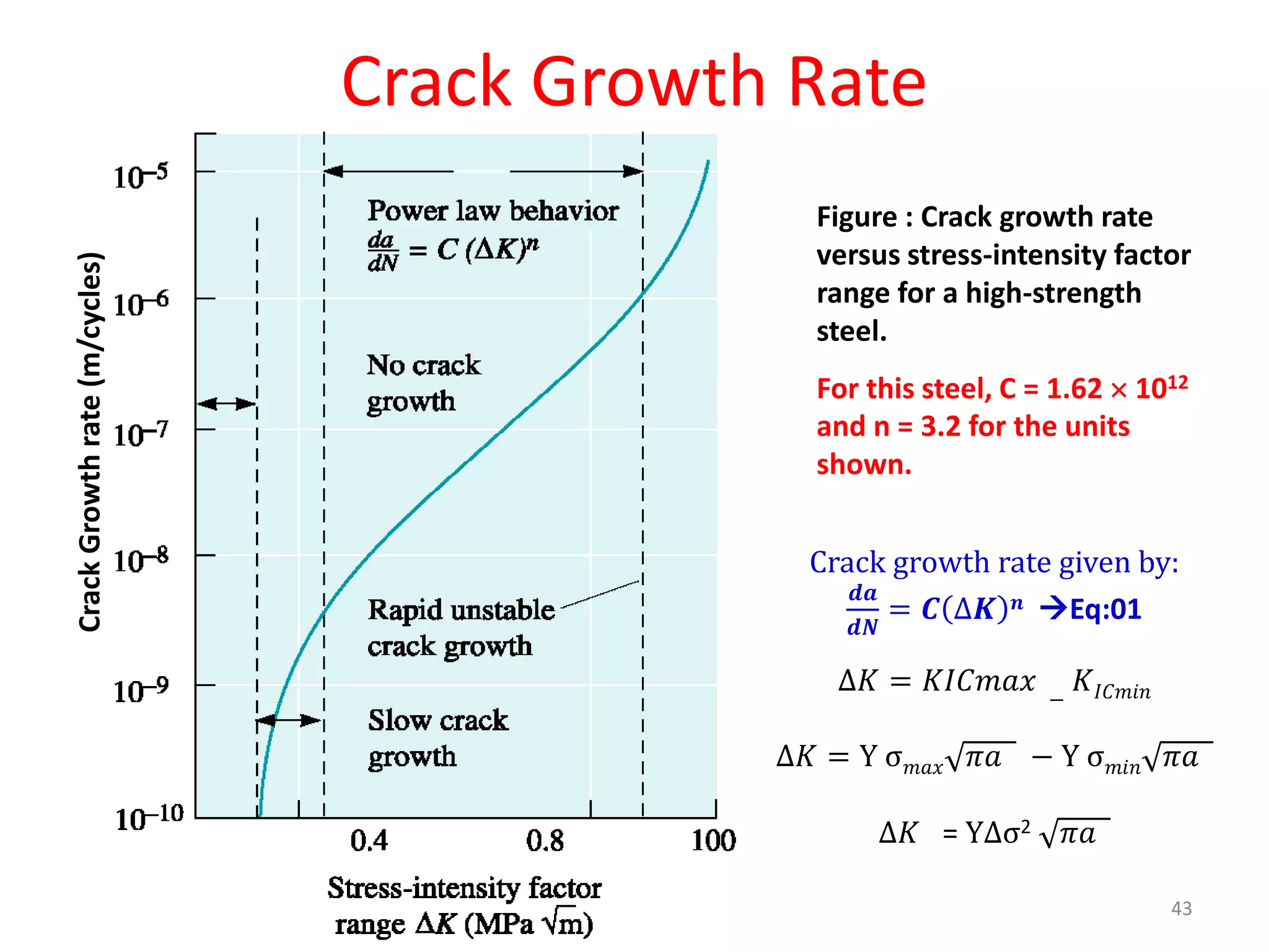
component and in nondestructive evaluation to determine if a crack
poses imminent danger to the structure.
• One approach to this problem is to estimate the number of cycle
required before failure occurs. By rearranging Equation 01 and
substituting for ∆𝐾: and integrate this b/w the initial size of the crack
and the crack size required for fracture to occur, we find that.
𝑁 =
2[(𝑎 𝑐)
2−𝑛
2 − 𝑎𝑖
2−𝑛
2 ]
2 − 𝑛 𝐶Y 𝑛∆σ 𝑛π 𝑛/2
• ai = initial Flaw size
• ac = flaw size required to fracture.
• C and n = are empirical constant depends upon the material.
45](https://image.slidesharecdn.com/fatigue-160316060415/75/Fracture-Mechanics-Failure-Analysis-Lecture-Fatigue-45-2048.jpg)


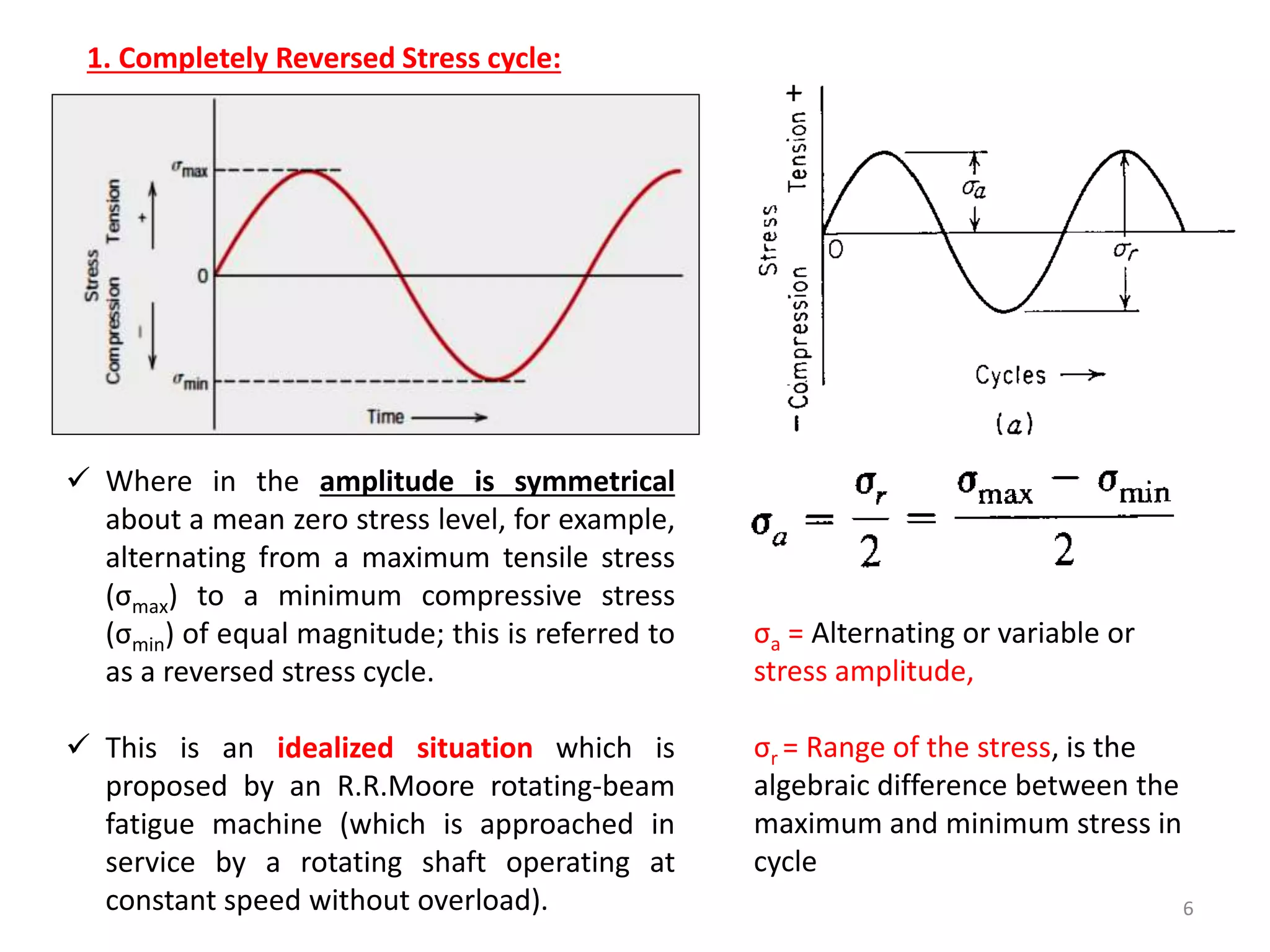
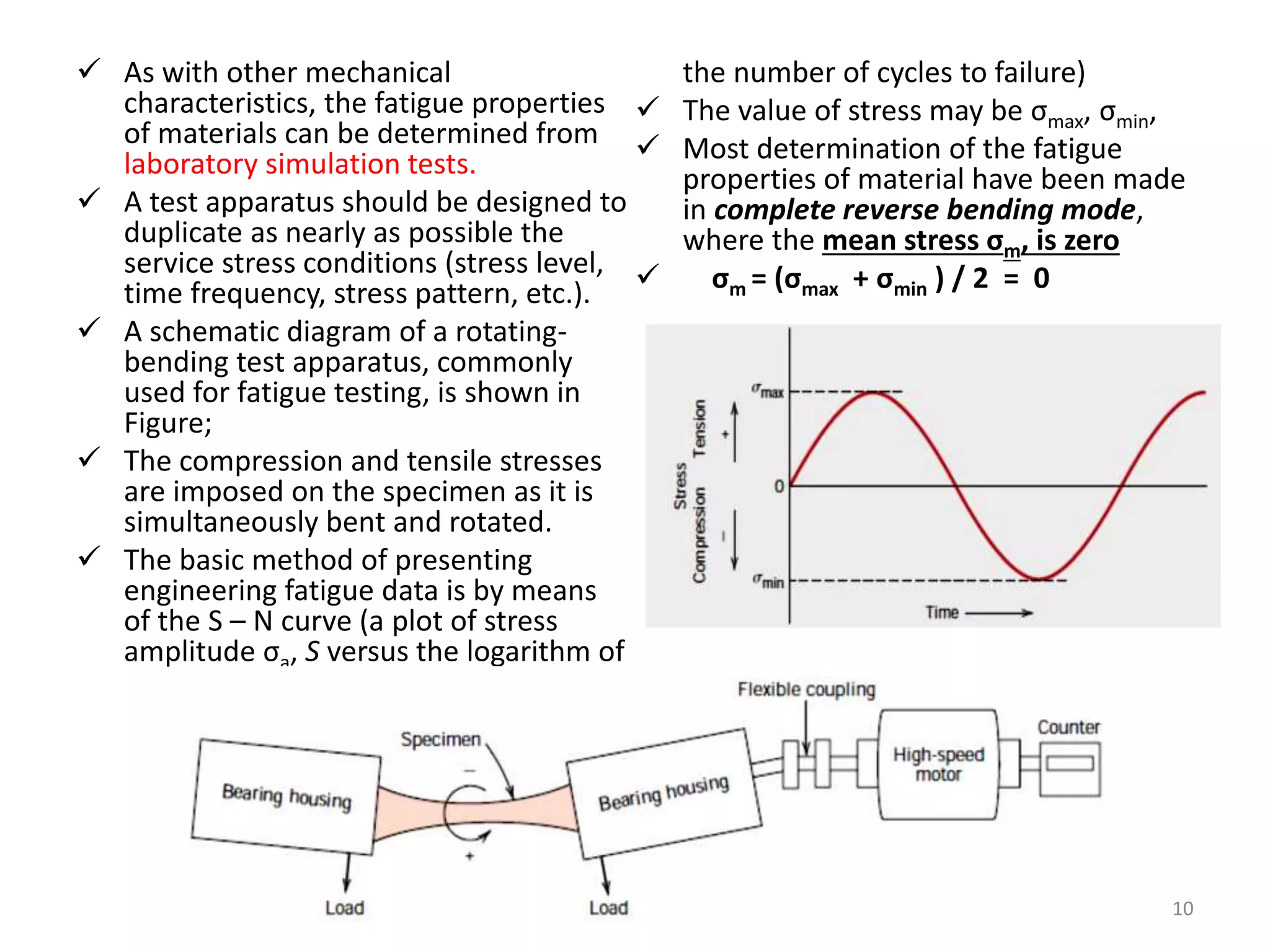
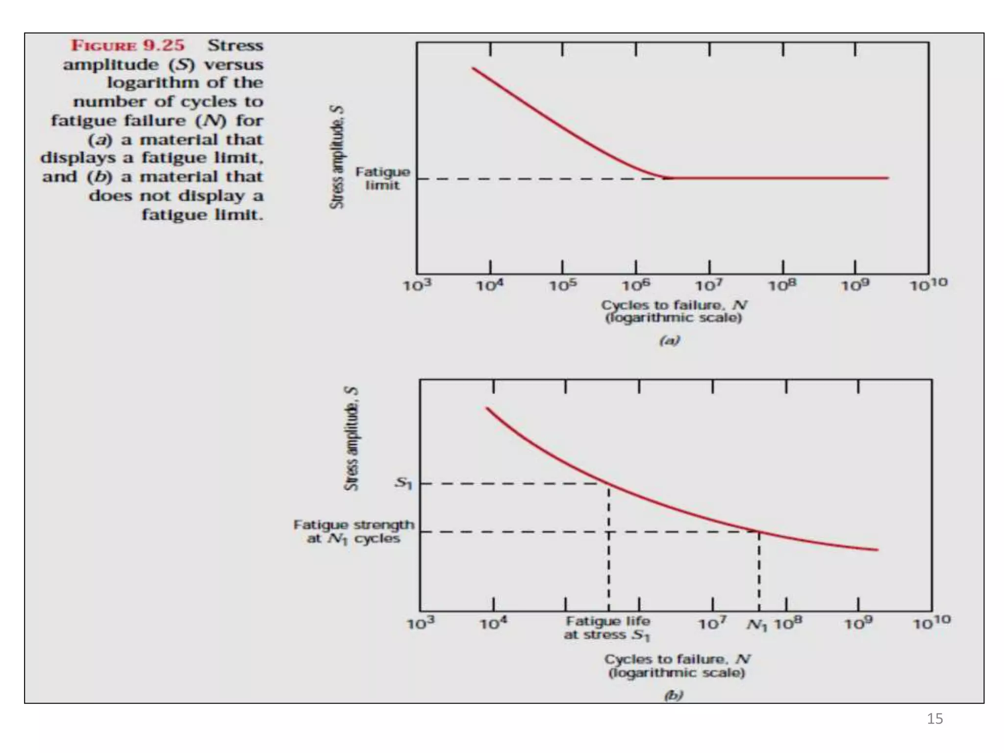
This document provides an introduction to fatigue, including: - Fatigue occurs when a component is subjected to fluctuating stresses and fails at a stress lower than its static strength. - It accounts for 90% of mechanical failures and occurs suddenly without warning. - Three factors are needed for fatigue failure: a maximum stress, stress variation, and sufficient number of cycles. - Fatigue testing involves subjecting specimens to cyclic stresses and recording the number of cycles until failure to generate an S-N curve.


