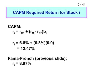
The Fama-French model predicts a lower required return for this stock compared to the CAPM. This is because the Fama-French model accounts for additional factors beyond just market risk.

1. 5-1
CHAPTER 5
Risk and Return: Portfolio Theory and
Asset Pricing Models
 Portfolio Theory
 Capital Asset Pricing Model (CAPM)
Efficient frontier
Capital Market Line (CML)
Security Market Line (SML)
Beta calculation
 Arbitrage pricing theory
 Fama-French 3-factor model

2. 5-2
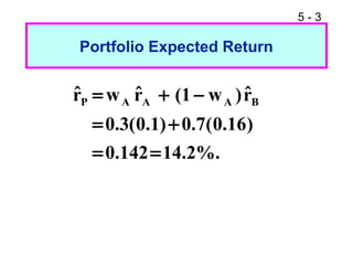
Portfolio Theory
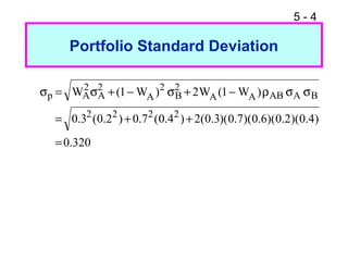
 Suppose Asset A has an expected return
of 10 percent and a standard deviation of
20 percent. Asset B has an expected
return of 16 percent and a standard
deviation of 40 percent. If the correlation
between A and B is 0.6, what are the
expected return and standard deviation for
a portfolio comprised of 30 percent Asset
A and 70 percent Asset B?

3. 5-3
Portfolio Expected Return
rP = w A rA + (1 − w A ) rB
ˆ ˆ ˆ
= 0.3( 0.1) + 0.7( 0.16)
= 0.142 = 14.2%.

4. 5-4
Portfolio Standard Deviation
σp = WA σ2 + (1 − WA )2 σ2 + 2WA (1 − WA ) ρAB σA σ B
2
A B
= 0.32 (0.22 ) + 0.72 (0.42 ) + 2(0.3)( 0.7)(0.6)(0.2)(0.4)
= 0.320

5. 5-5
Attainable Portfolios: ρ AB = 0.4
ρ AB = +0.4: Attainable Set of
Risk/Return Combinations
20%
15%
Expected return
10%
5%
0%
0% 10% 20% 30% 40%
Risk, σ p

6. 5-6
Attainable Portfolios: ρ AB = +1
ρ AB = +1.0: Attainable Set of Risk/Return
Combinations
20%
Expected return
15%
10%
5%
0%
0% 10% 20% 30% 40%
Risk, σ p

7. 5-7
Attainable Portfolios: ρ AB = -1
ρ AB = -1.0: Attainable Set of Risk/Return
Combinations
20%
Expected return
15%
10%
5%
0%
0% 10% 20% 30% 40%
Risk, σ p

8. 5-8
Attainable Portfolios with Risk-Free
Asset (Expected risk-free return = 5%)
Attainable Set of Risk/Return
Combinations with Risk-Free Asset
15%
Expected return
10%
5%
0%
0% 5% 10% 15% 20%
Risk, σp

9. 5-9
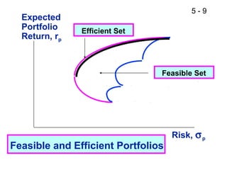
Expected
Portfolio Efficient Set
Return, rp
Feasible Set
Risk, σ p
Feasible and Efficient Portfolios

10. 5 - 10
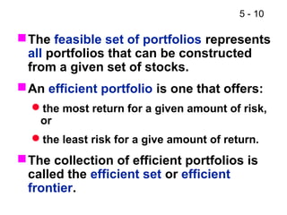
 The feasible set of portfolios represents
all portfolios that can be constructed
from a given set of stocks.
 An efficient portfolio is one that offers:
the most return for a given amount of risk,
or
the least risk for a give amount of return.
 The collection of efficient portfolios is
called the efficient set or efficient
frontier.

11. 5 - 11
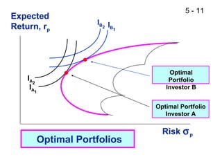
Expected
IB2 I
Return, rp B 1
Optimal
IA2 Portfolio
IA1 Investor B
Optimal Portfolio
Investor A
Risk σ p
Optimal Portfolios

12. 5 - 12
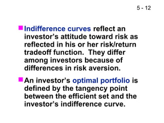
 Indifference curves reflect an
investor’s attitude toward risk as
reflected in his or her risk/return
tradeoff function. They differ
among investors because of
differences in risk aversion.
 An investor’s optimal portfolio is
defined by the tangency point
between the efficient set and the
investor’s indifference curve.

13. 5 - 13
What is the CAPM?
 The CAPM is an equilibrium model
that specifies the relationship
between risk and required rate of
return for assets held in well-
diversified portfolios.
 It is based on the premise that only
one factor affects risk.
 What is that factor?

14. 5 - 14
What are the assumptions
of the CAPM?
 Investors all think in terms of
a single holding period.
 All investors have identical expectations.
 Investors can borrow or lend unlimited
amounts at the risk-free rate.
(More...)

15. 5 - 15
 All assets are perfectly divisible.
 There are no taxes and no transactions
costs.
 All investors are price takers, that is,
investors’ buying and selling won’t
influence stock prices.
 Quantities of all assets are given and
fixed.

16. 5 - 16
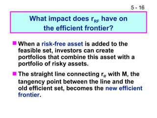
What impact does rRF have on
the efficient frontier?
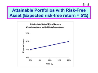
 When a risk-free asset is added to the
feasible set, investors can create
portfolios that combine this asset with a
portfolio of risky assets.
 The straight line connecting rRF with M, the
tangency point between the line and the
old efficient set, becomes the new efficient
frontier.

17. 5 - 17
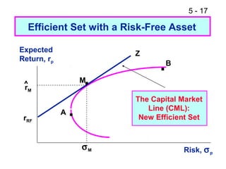
Efficient Set with a Risk-Free Asset
Expected Z
Return, rp
. B
^
rM
.
M
The Capital Market
rRF
A . Line (CML):
New Efficient Set
σM Risk, σ p

18. 5 - 18
What is the Capital Market Line?
 The Capital Market Line (CML) is all
linear combinations of the risk-free
asset and Portfolio M.
 Portfolios below the CML are inferior.
The CML defines the new efficient set.
All investors will choose a portfolio on
the CML.

19. 5 - 19
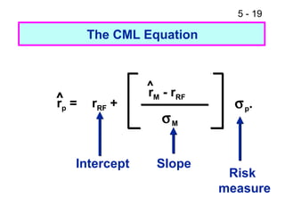
The CML Equation
^
rM - rRF
^=
rp rRF + σ p.
σM
Intercept Slope
Risk
measure

20. 5 - 20
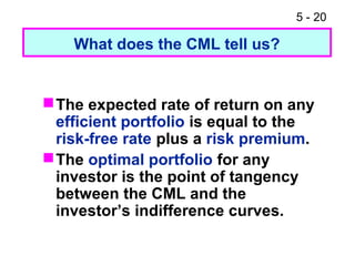
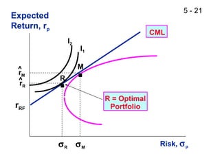
What does the CML tell us?
 The expected rate of return on any
efficient portfolio is equal to the
risk-free rate plus a risk premium.
 The optimal portfolio for any
investor is the point of tangency
between the CML and the
investor’s indifference curves.

21. 5 - 21
Expected
Return, rp
CML
I2
I1
^
rM
^
r R .
R
. M
R = Optimal
rRF Portfolio
σR σM Risk, σ p

22. 5 - 22
What is the Security Market Line (SML)?
 The CML gives the risk/return
relationship for efficient portfolios.
 The Security Market Line (SML), also
part of the CAPM, gives the risk/return
relationship for individual stocks.

23. 5 - 23
The SML Equation
 The measure of risk used in the SML
is the beta coefficient of company i, bi.
 The SML equation:
ri = rRF + (RPM) bi

24. 5 - 24
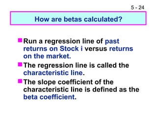
How are betas calculated?
 Run a regression line of past
returns on Stock i versus returns
on the market.
 The regression line is called the
characteristic line.
 The slope coefficient of the
characteristic line is defined as the
beta coefficient.

25. 5 - 25
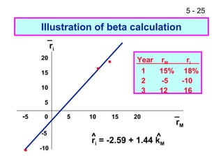
Illustration of beta calculation
_
ri
20
. . Year rM ri
15 1 15% 18%
2 -5 -10
10
3 12 16
5
-5 0 5 10 15 20 _
rM
-5
^ = -2.59 + 1.44 k
ri ^
. -10
M

26. 5 - 26
Method of Calculation
 Analysts use a computer with
statistical or spreadsheet software to
perform the regression.
At least 3 year’s of monthly returns or 1
year’s of weekly returns are used.
Many analysts use 5 years of monthly
returns.
(More...)

27. 5 - 27
 If beta = 1.0, stock is average risk.
 If beta > 1.0, stock is riskier than
average.
 If beta < 1.0, stock is less risky than
average.
 Most stocks have betas in the range
of 0.5 to 1.5.

28. 5 - 28
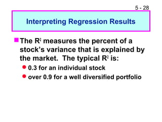
Interpreting Regression Results
 The R2 measures the percent of a
stock’s variance that is explained by
the market. The typical R2 is:
0.3 for an individual stock
over 0.9 for a well diversified portfolio

29. 5 - 29
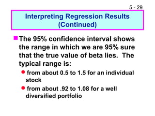
Interpreting Regression Results
(Continued)
 The 95% confidence interval shows
the range in which we are 95% sure
that the true value of beta lies. The
typical range is:
from about 0.5 to 1.5 for an individual
stock
from about .92 to 1.08 for a well
diversified portfolio

30. 5 - 30
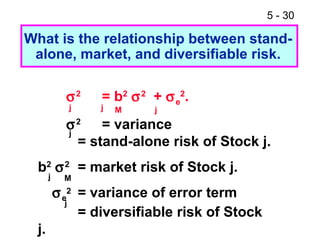
What is the relationship between stand-
alone, market, and diversifiable risk.
σ2 = b2 σ 2 + σ e2.
j j M j
σ 2 = variance
j
= stand-alone risk of Stock j.
b2 σ 2 = market risk of Stock j.
j M
σ e2 = variance of error term
j
= diversifiable risk of Stock
j.

31. 5 - 31
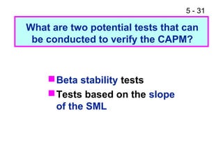
What are two potential tests that can
be conducted to verify the CAPM?
 Beta stability tests
 Tests based on the slope
of the SML

32. 5 - 32
Tests of the SML indicate:
 A more-or-less linear relationship
between realized returns and market
risk.
 Slope is less than predicted.
 Irrelevance of diversifiable risk
specified in the CAPM model can be
questioned.
(More...)

33. 5 - 33
 Betas of individual securities are not
good estimators of future risk.
 Betas of portfolios of 10 or more
randomly selected stocks are
reasonably stable.
 Past portfolio betas are good
estimates of future portfolio
volatility.

34. 5 - 34
Are there problems with the
CAPM tests?
 Yes.
Richard Roll questioned whether it
was even conceptually possible to test
the CAPM.
Roll showed that it is virtually
impossible to prove investors behave
in accordance with CAPM theory.

35. 5 - 35
What are our conclusions
regarding the CAPM?
 It is impossible to verify.
 Recent studies have questioned its
validity.
 Investors seem to be concerned with
both market risk and stand-alone
risk. Therefore, the SML may not
produce a correct estimate of ri. (More...)

36. 5 - 36
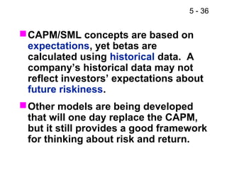
 CAPM/SML concepts are based on
expectations, yet betas are
calculated using historical data. A
company’s historical data may not
reflect investors’ expectations about
future riskiness.
 Other models are being developed
that will one day replace the CAPM,
but it still provides a good framework
for thinking about risk and return.

37. 5 - 37
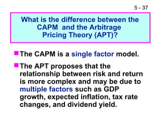
What is the difference between the
CAPM and the Arbitrage
Pricing Theory (APT)?
 The CAPM is a single factor model.
 The APT proposes that the
relationship between risk and return
is more complex and may be due to
multiple factors such as GDP
growth, expected inflation, tax rate
changes, and dividend yield.

38. 5 - 38
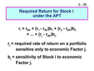
Required Return for Stock i
under the APT
ri = rRF + (r1 - rRF)b1 + (r2 - rRF)b2
+ ... + (rj - rRF)bj.
rj = required rate of return on a portfolio
sensitive only to economic Factor j.
bj = sensitivity of Stock i to economic
Factor j.

39. 5 - 39
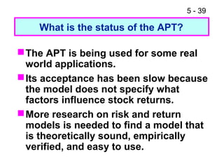
What is the status of the APT?
 The APT is being used for some real
world applications.
 Its acceptance has been slow because
the model does not specify what
factors influence stock returns.
 More research on risk and return
models is needed to find a model that
is theoretically sound, empirically
verified, and easy to use.

40. 5 - 40
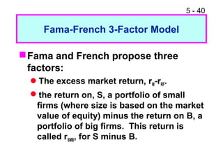
Fama-French 3-Factor Model
 Fama and French propose three
factors:
The excess market return, rM-rRF.
the return on, S, a portfolio of small
firms (where size is based on the market
value of equity) minus the return on B, a
portfolio of big firms. This return is
called rSMB, for S minus B.

41. 5 - 41
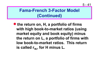
Fama-French 3-Factor Model
(Continued)
the return on, H, a portfolio of firms
with high book-to-market ratios (using
market equity and book equity) minus
the return on L, a portfolio of firms with
low book-to-market ratios. This return
is called rHML, for H minus L.

42. 5 - 42
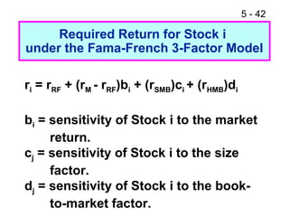
Required Return for Stock i
under the Fama-French 3-Factor Model
ri = rRF + (rM - rRF)bi + (rSMB)ci + (rHMB)di
bi = sensitivity of Stock i to the market
return.
cj = sensitivity of Stock i to the size
factor.
dj = sensitivity of Stock i to the book-
to-market factor.

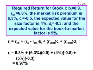
43. 5 - 43
Required Return for Stock i: bi=0.9,
rRF=6.8%, the market risk premium is
6.3%, ci=-0.5, the expected value for the
size factor is 4%, di=-0.3, and the
expected value for the book-to-market
factor is 5%.
ri = rRF + (rM - rRF)bi + (rSMB)ci + (rHMB)di
ri = 6.8% + (6.3%)(0.9) + (4%)(-0.5) +
(5%)(-0.3)
= 8.97%

44. 5 - 44
CAPM Required Return for Stock i
CAPM:
ri = rRF + (rM - rRF)bi
ri = 6.8% + (6.3%)(0.9)
= 12.47%
Fama-French (previous slide):
ri = 8.97%