Downloaded 304 times

![COVARIANCE OF RISK-FREE ASSET WITH A RISKY
ASSET
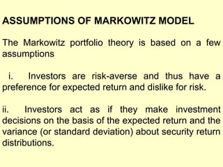
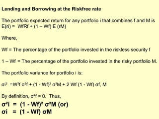
The covariance between two sets of returns, A and B where
asset A is a risk free asset.
n
CovAB
= Σ[rA- E(rA)] [ rB - E(rB)]/n
A=1
The uncertainty for a risk-free asset is known, so σA=0,
which implies that rA = E(rA) for all the periods. Thus, rA E(rA) =0, which further leads to the facts that the product of
any other expressions with this expression will be zero. This
will result in the covariance of the risk-free asset with any
risky asset or portfolio to be also zero. Similarly, the
correlation between any risky asset and risk-free asset, will](https://image.slidesharecdn.com/capitalmarkettheory-131030042348-phpapp01/85/Capital-market-theory-11-320.jpg)
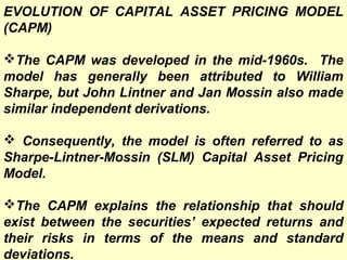
![RISK-RETURN POSSIBILITIES WITH LEVERAGE
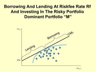
An investor always wants to increase his expected
returns. Say, a person has borrowed an amount
which is 50 percent of his original wealth, the effect of
this on the expected return for the portfolio would be:
E(ri)
= Wf (rf) + (1 - Wf) E(rk) where k is the
risky assets portfolio
= – 0.50 (rf) + [1 – (–0.50)] E(rk)
= – 0.50 (rf) + 1.50 E(rk)
Continued](https://image.slidesharecdn.com/capitalmarkettheory-131030042348-phpapp01/85/Capital-market-theory-13-320.jpg)
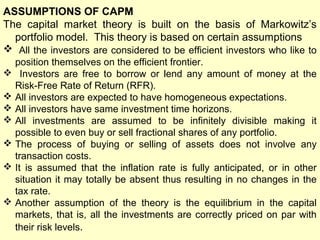
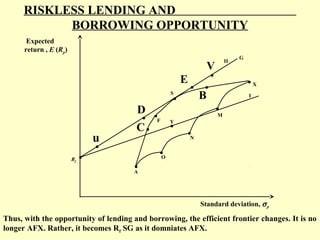
![Thus, we see that the return increases in a linear fashion
along the line of risk-free rate (rf) and ‘k’.
Now, suppose E(rf) = 0.10
And E(rk) = 0.24
E(ri) = = – 0.50 (0.10) + 1.5 (0.24) = 0.31 or 31%
Similar is the effect of standard deviation of the
leveraged portfolio.
E(σi) = (1 – Wf) σk
= [1 – (–0.5)] σk = 1.50 σk](https://image.slidesharecdn.com/capitalmarkettheory-131030042348-phpapp01/85/Capital-market-theory-14-320.jpg)

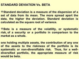
![Explanation:
The CAPM states that the expected return of a security
or a portfolio equals the rate on a risk-free security plus
a risk premium. If this expected return does not meet or
beat the required return, then the investment should not
be undertaken. The security market line plots the results
of the CAPM for all different risks (betas).
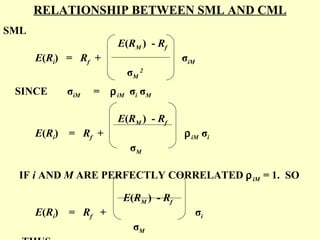
thus the CML is important in describing the
equilibrium relationship between expected return and
risk for efficient portfolios that contains no unsystematic
risk.
Thus as per the CAPM model, the expected return of
any asset is given by a formula of the form:
E[ri] = rf + [Number of Units of Risk][Risk Premium per
Unit]](https://image.slidesharecdn.com/capitalmarkettheory-131030042348-phpapp01/85/Capital-market-theory-26-320.jpg)
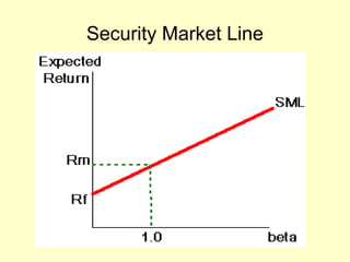
![SECURITY MARKET LINE (SML)
The SML essentially graphs the results from the capital
asset pricing model (CAPM) formula. The x-axis
represents the risk (beta), and the y-axis represents
the expected return. The market risk premium is
determined from the slope of the SML.
E (R i ) = R f + [ E (R M) - R f ] β i](https://image.slidesharecdn.com/capitalmarkettheory-131030042348-phpapp01/85/Capital-market-theory-27-320.jpg)

![TESTS OF ASSET PRICING THEORIES
The CAPM pricing model is given by the
equation:
E(ri) = rf + [E(rM) – rf] βi
According to the theory, the expected return on
security i, E(ri), is related to the risk-free rate, rf,
plus a risk premium, [E(rM) – rf] βi ,which
includes the expected return on the market
portfolio.](https://image.slidesharecdn.com/capitalmarkettheory-131030042348-phpapp01/85/Capital-market-theory-32-320.jpg)

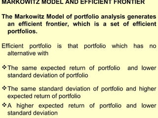
The Markowitz model generates an efficient frontier of optimal portfolios that maximize return for a given level of risk. The Capital Asset Pricing Model (CAPM) builds on this by deriving the security market line (SML) which plots the expected return of individual securities based on their beta coefficient in relation to the market portfolio. The capital market line (CML) extends the efficient frontier by including a risk-free asset, demonstrating how investors can optimize the trade-off between risk and return through borrowing and lending at the risk-free rate.


![APT_&_VaR[1]](https://cdn.slidesharecdn.com/ss_thumbnails/9cf85d63-155b-48fb-9bf9-2eef1776ff5f-150626091222-lva1-app6892-thumbnail.jpg?width=640&height=640&fit=bounds)


