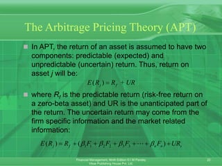
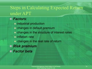
Risk-Return Models and Portfolio Theory

Chapter - 5
Risk and Return: Portfolio
Theory and Assets Pricing
Models

2
Financial Management, Ninth Edition © I M Pandey
Vikas Publishing House Pvt. Ltd.
Chapter Objectives
 Discuss the concepts of portfolio risk and
return.
 Determine the relationship between risk and
return of portfolios.
 Highlight the difference between systematic
and unsystematic risks.
 Examine the logic of portfolio theory .
 Show the use of capital asset pricing model
(CAPM) in the valuation of securities.
 Explain the features and modus operandi of
the arbitrage pricing theory (APT).

3
Introduction
 A portfolio is a bundle or a combination of
individual assets or securities.
 The portfolio theory provides a normative
approach to investors to make decisions to
invest their wealth in assets or securities
under risk.
 It is based on the assumption that investors are
risk-averse.
 The second assumption of the portfolio theory is
that the returns of assets are normally distributed.

4
Portfolio Return: Two-Asset Case
 The return of a portfolio is equal to the
weighted average of the returns of individual
assets (or securities) in the portfolio with
weights being equal to the proportion of
investment value in each asset.
Expected return on portfolio weight of security × expected return on security
weight of security × expected return on security
X X
Y Y



5
Portfolio Risk: Two-Asset Case
 The portfolio variance or standard deviation depends
on the co-movement of returns on two assets.
Covariance of returns on two assets measures their
co-movement.
 The formula for calculating covariance of returns of
the two securities X and Y is as follows:
Covariance XY = Standard deviation X ´ Standard
deviation Y ´ Correlation XY
 The variance of two-security portfolio is given by the
following equation:
2 2 2 2 2
2 2 2 2
2 Covar
2 Cor
p x x y y x y xy
x x y y x y x y xy
w w w w
w w w w
  
   
  
  

6
Minimum Variance Portfolio
 w* is the optimum proportion of investment in
security X. Investment in Y will be: 1 – w*.
2
2 2
Cov
*
2Cov
y xy
x y xy
w

 


 

7
Portfolio Risk Depends on Correlation
between Assets
 When correlation coefficient of returns on
individual securities is perfectly positive (i.e.,
cor = 1.0), then there is no advantage of
diversification.
 The weighted standard deviation of returns
on individual securities is equal to the
standard deviation of the portfolio.
 We may therefore conclude that
diversification always reduces risk provided
the correlation coefficient is less than 1.

8
Portfolio Return and Risk for
Different Correlation Coefficients
Portfolio Risk, p (%)
Correlation
Weight
Portfolio
Return (%) +1.00 -1.00 0.00 0.50 -0.25
Logrow Rapidex Rp p p p p p
1.00 0.00 12.00 16.00 16.00 16.00 16.00 16.00
0.90 0.10 12.60 16.80 12.00 14.60 15.74 13.99
0.80 0.20 13.20 17.60 8.00 13.67 15.76 12.50
0.70 0.30 13.80 18.40 4.00 13.31 16.06 11.70
0.60 0.40 14.40 19.20 0.00 13.58 16.63 11.76
0.50 0.50 15.00 20.00 4.00 14.42 17.44 12.65
0.40 0.60 15.60 20.80 8.00 15.76 18.45 14.22
0.30 0.70 16.20 21.60 12.00 17.47 19.64 16.28
0.20 0.80 16.80 22.40 16.00 19.46 20.98 18.66
0.10 0.90 17.40 23.20 20.00 21.66 22.44 21.26
0.00 1.00 18.00 24.00 24.00 24.00 24.00 24.00
Minimum Variance Portfolio
wL 1.00 0.60 0.692 0.857 0.656
wR 0.00 0.40 0.308 0.143 0.344
2
256 0.00 177.23 246.86 135.00
 (%) 16 0.00 13.31 15.71 11.62

9
Investment Opportunity Sets (2 Assets)
given Different Correlations
0
5
10
15
20
0 5 10 15 20 25 30
Porfolio risk (Stdev, %)
Portfolio
return,
%
Cor = - 1.0
Cor = - 0.25
Cor = + 1.0
Cor = + 0.50
Cor = - 1.0
L
R

10
Mean-Variance Criterion
 A risk-averse investor will prefer a portfolio
with the highest expected return for a given
level of risk or prefer a portfolio with the
lowest level of risk for a given level of
expected return. In portfolio theory, this is
referred to as the principle of dominance.

11
Investment Opportunity Set:
The N-Asset Case
 An efficient portfolio
is one that has the
highest expected
returns for a given level
of risk. The efficient
frontier is the frontier
formed by the set of
efficient portfolios. All
other portfolios, which
lie outside the efficient
frontier, are inefficient
portfolios.
Risk, 
Return
A
P
Q
B
C
D
x
x
x
x
x
x
x
R

12
Risk Diversification: Systematic
and Unsystematic Risk
 Risk has two parts:
 Systematic risk arises on account of the economy-wide
uncertainties and the tendency of individual securities to move
together with changes in the market. This part of risk cannot be
reduced through diversification. It is also known as market
risk.
 Unsystematic risk arises from the unique uncertainties of
individual securities. It is also called unique risk. Unsystematic
risk can be totally reduced through diversification.
 Total risk = Systematic risk + Unsystematic risk
 Systematic risk is the covariance of the individual
securities in the portfolio. The difference between variance
and covariance is the diversifiable or unsystematic risk.

13
A Risk-Free Asset and a Risky Asset
 A risk-free asset or security has a zero
variance or standard deviation.
 Return and risk when we combine a risk-free
and a risky asset:
( ) ( ) (1 )
p j f
E R wE R w R
  
p j
w
 


14
A Risk-Free Asset and
A Risky Asset: Example
RISK-RETURN ANALYSIS FOR A PORTFOLIO OF A RISKY AND A RISK-FREE SECURITIES
Weights (%) Expected Return, Rp
Standard Deviation (p)
Risky security Risk-free security (%) (%)
120 – 20 17 7.2
100 0 15 6.0
80 20 13 4.8
60 40 11 3.6
40 60 9 2.4
20 80 7 1.2
0 100 5 0.0
0
2.5
5
7.5
10
12.5
15
17.5
20
0 1.8 3.6 5.4 7.2 9
Standard Deviation
Expected
Return
A
B
C
D
Rf, risk-free rate

15
Multiple Risky Assets and
A Risk-Free Asset
 We can combine earlier
figures to illustrate the
feasible portfolios consisting
of the risk-free security and
the portfolios of risky
securities.
 We draw three lines from the
risk-free rate (5%) to three
portfolios. Each line shows
the manner in which capital
is allocated. This line is
called the capital allocation
line (CAL).
 The capital market line
(CML) is an efficient set of
risk-free and risky securities,
and it shows the risk-return
trade-off in the market
equilibrium.
Risk, 
Return
B
M
Q
(
N
O
L
R
Capital Market Line (CML)
Capital Allocation Lines
(CALs)
P

16
Capital Market Line
 The slope of CML describes the best price of
a given level of risk in equilibrium.
 The expected return on a portfolio on CML is
defined by the following equation:
( )
Slope of CML
m f
m
E R R


 
  
 
( )
( )
m f
p f p
m
E R R
E R R 


 
   
 

17
Capital Asset Pricing Model (CAPM)
 The capital asset pricing model (CAPM) is
a model that provides a framework to
determine the required rate of return on an
asset and indicates the relationship between
return and risk of the asset.
 Assumptions of CAPM
 Market efficiency
 Risk aversion and mean-variance optimisation
 Homogeneous expectations
 Single time period
 Risk-free rate

18
Characteristics Line: Market
Return vs. Alpha’s Return
 We plot the combinations of
four possible returns of
Alpha and market. They are
shown as four points. The
combinations of the
expected returns points
(22.5%, 27.5% and –12.5%,
20%) are also shown in the
figure. We join these two
points to form a line. This
line is called the
characteristics line. The
slope of the characteristics
line is the sensitivity
coefficient, which, as stated
earlier, is referred to as
beta.
-30.0
-25.0
-20.0
-15.0
-10.0
-5.0
0.0
5.0
10.0
15.0
20.0
25.0
30.0
35.0
-20.0 -15.0 -10.0 -5.0 0.0 5.0 10.0 15.0 20.0 25.0 30.0
Market
Return
Alpha's
Return
*
*

19
Security Market Line (SML)
 For a given amount of systematic risk (),
SML shows the required rate of return.
 = (covarj,m/2
m)
SLM
E(Rj)
Rm
Rf
1.0
0
 
j f m f j
E(R ) = R + (R ) – R β

20
Implications of CAPM
 Investors will always combine a risk-free asset with a
market portfolio of risky assets. They will invest in risky
assets in proportion to their market value.
 Investors will be compensated only for that risk which
they cannot diversify. This is the market-related
(systematic) risk.
 Beta, which is a ratio of the covariance between the
asset returns and the market returns divided by the
market variance, is the most appropriate measure of
an asset’s risk.
 Investors can expect returns from their investment
according to the risk. This implies a linear relationship
between the asset’s expected return and its beta.

21
Limitations of CAPM
 It is based on unrealistic assumptions.
 It is difficult to test the validity of CAPM.
 Betas do not remain stable over time.

22
The Arbitrage Pricing Theory (APT)
 In APT, the return of an asset is assumed to have two
components: predictable (expected) and
unpredictable (uncertain) return. Thus, return on
asset j will be:
 where Rf is the predictable return (risk-free return on
a zero-beta asset) and UR is the unanticipated part of
the return. The uncertain return may come from the
firm specific information and the market related
information:
( ) +
j f
E R R UR

1 1 2 2 3 3
( ) ( )
j f n n s
E R R F F F F UR
   
      

23
Steps in Calculating Expected Return
under APT
 Factors:
 industrial production
 changes in default premium
 changes in the structure of interest rates
 inflation rate
 changes in the real rate of return
 Risk premium
 Factor beta

Risk-Return Models and Portfolio Theory

Recommended

Recommended

More Related Content

Similar to Risk-Return Models and Portfolio Theory

Similar to Risk-Return Models and Portfolio Theory (20)

More from kemboies

More from kemboies (7)

Recently uploaded

Recently uploaded (20)

Risk-Return Models and Portfolio Theory