Downloaded 476 times
![Suggested Readings
Reference 1 Reference 2
2
Chapter 10 of Ref [1], Chapter 6 of Ref [2], Chapter 4 of Ref [3]
Reference 3](https://image.slidesharecdn.com/lec10lec11fatigueanalysis-161211121313/85/Fatigue-Analysis-of-Structures-Aerospace-Application-2-320.jpg)


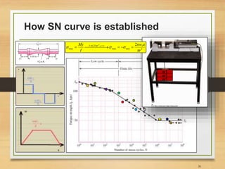
![Output from fatigue test (see Ref [3])
23
The number of cycles to failure is called
fatigue life Nf
Each cycle is equal
to two reversals
Stress in the component some
books use symbol σ instead
time
Stress](https://image.slidesharecdn.com/lec10lec11fatigueanalysis-161211121313/85/Fatigue-Analysis-of-Structures-Aerospace-Application-23-320.jpg)
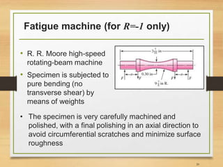
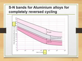
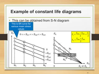
![S-N/Wohler diagram (see Ref [2])
25
Results of completely
reversed axial fatigue tests.
Material: UNS G41300 steel,
normalized; Sut = 116 kpsi;
maximum Sut = 125 kpsi.
Often plotted in log-log or semi-log graphs. If
plotted in log-log, y axis is in terms of stress
amplitude or stress range and x axis in terms
of number of reversals or cycles to failure](https://image.slidesharecdn.com/lec10lec11fatigueanalysis-161211121313/85/Fatigue-Analysis-of-Structures-Aerospace-Application-25-320.jpg)
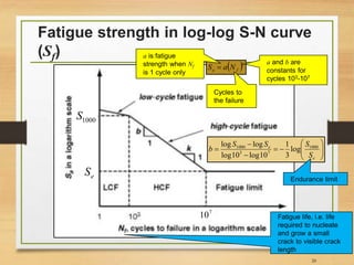
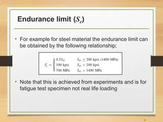
![Endurance limit (Se)
• In real life endurance limit can be different due to
many factors (see Ref [2] for more details);
33](https://image.slidesharecdn.com/lec10lec11fatigueanalysis-161211121313/85/Fatigue-Analysis-of-Structures-Aerospace-Application-33-320.jpg)


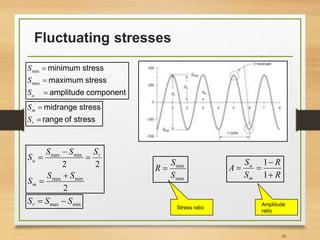
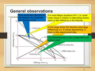
![Important Notes [3]
• Fatigue damage of components correlates strongly with;
• Applied stress amplitude/range
• Applied mean stress (mostly in high cycle fatigue region)
• In high cycle fatigue, direct (normal) mean stress is
responsible for opening and closing micro-cracks
• Normal tensile mean stresses are detrimental and
compressive mean stress are beneficial for fatigue
strength (why?)
• Shear mean stress has little effect on crack propagation
• There is no/little effect of mean stress in low cycle fatigue
due to large amount of plastic deformation
81](https://image.slidesharecdn.com/lec10lec11fatigueanalysis-161211121313/85/Fatigue-Analysis-of-Structures-Aerospace-Application-81-320.jpg)
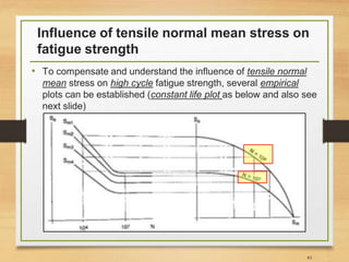
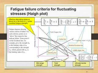
![Important Notes [3]
• So far, what we have been doing was based on not taking
into account the effects of tensile normal mean stresses on
the high cycle fatigue strength of components
• We have been assuming Sm=0
• Therefore, below scientists proposed empirical equations
to take such effect into account;
• Gerber (1874)
• Goodman (1899)
• Haigh (1917)
• Soderberg (1930)
82](https://image.slidesharecdn.com/lec10lec11fatigueanalysis-161211121313/85/Fatigue-Analysis-of-Structures-Aerospace-Application-82-320.jpg)
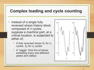
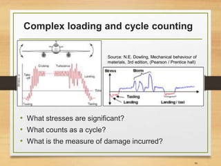
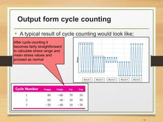
![Methods of cycle counting
• Beyond the scope of this lecture
• Interested readers are recommended to refer to
chapter 3 of Ref. [3];
• Level crossing cycle counting
• Peak-valley cycle counting
• Range counting
• Three-point cycle counting method
• Four-point cycle counting method
• Rain-flow counting technique
91](https://image.slidesharecdn.com/lec10lec11fatigueanalysis-161211121313/85/Fatigue-Analysis-of-Structures-Aerospace-Application-91-320.jpg)


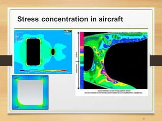
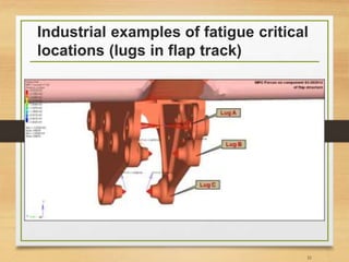
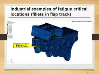
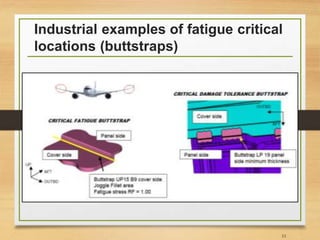
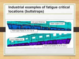
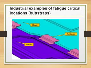
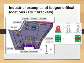
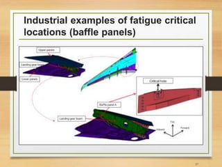
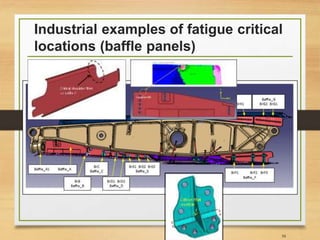
This document provides an introduction to fatigue analysis of aerospace structures. It discusses key topics including stress-life analysis methods, S-N curves, stress concentration factors, notch sensitivity, and fatigue failure locations. Examples of fatigue critical locations in aircraft components like flaps, struts, and baffle panels are also shown. The document concludes with examples calculating stresses, stress ratios, and fatigue life based on the stress-life approach.