The document discusses energy methods for structural analysis, including the total potential energy method. It provides examples of deriving the strain energy stored in different structural members under different loading conditions such as axial force, bending moment, shear force, and torsion. It also provides examples of using the principle of stationary total potential energy to solve for displacements in determinate structures by assuming a displacement function and minimizing the total potential energy.

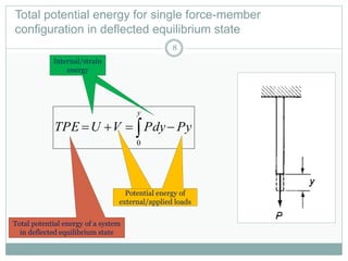
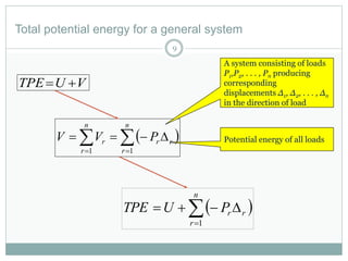
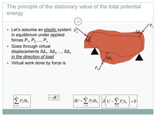
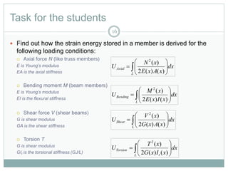
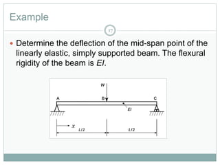
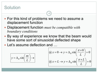
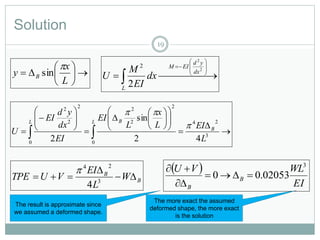
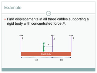
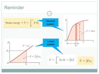
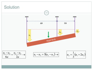
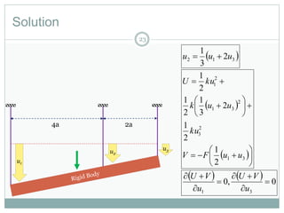
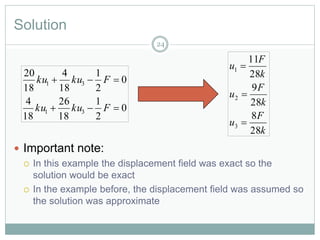
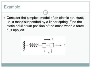
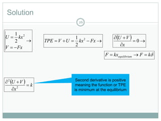
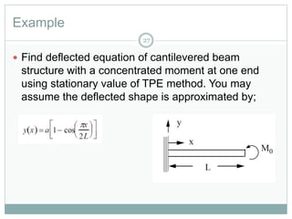
1. B Y
D R . M AH D I D AM G H AN I
2 0 1 6 - 2 0 1 7
Structural Design and
Inspection-Energy method
1

2. Suggested Readings
Reference 1 Reference 2
2

3. Objective(s)
 Familiarisation with Total Potential Energy (TPE)
 Familiarisation with stationary value of TPE
 Familiarisation with Rayleigh Ritz method
3

4. Review
4
 So far we have seen the following energy methods;
 Principle of virtual work
 Castigliano’s first theorem
 The first partial derivative of the total internal complimentary energy
in a structure with respect to any particular deflection component at a
point is equal to the force applied at that point and in the direction
corresponding to that deflection component.
 Castigliano’s second theorem
 The first partial derivative of the total internal energy in a structure
with respect to the force applied at any point is equal to the deflection
at the point of application of that force in the direction of its line of
action.
 Unit load theorem
 Unit displacement theorem
 Principle of complimentary energy

5. If instead of weight we had force
P then V=–Py (loss of energy).
Deflection can be associated
with the loss of potential energy.
Total Potential Energy (TPE)
Potential Energy of the
mass= Mgh
Potential Energy= Mg(h-y)
Loss of
energy for
-Mgy
In equilibrium
5
Arbitrary datum
In deflected equilibrium

6. Note
6
 Assuming that the potential energy of the system is
zero in the unloaded state, then the loss of potential
energy of the load P as it produces a deflection y is Py
 The potential energy V of P in the deflected equilibrium
state is given by;
00  PhorMghassume

7. Note (strain energy in a system)
7

y
PdyU
0
Strain energy
produced by
load P

8. Total potential energy for single force-member
configuration in deflected equilibrium state
PyPdyVUTPE
y
 0
Total potential energy of a system
in deflected equilibrium state
Internal/strain
energy
Potential energy of
external/applied loads
Potential energy of
external/applied loads
Internal/strain
energy
8

9. Total potential energy for a general system
VUTPE 
  

n
r
rr
n
r
r PVV
11
A system consisting of loads
P1,P2, . . . , Pn producing
corresponding
displacements Δ1, Δ2, . . . , Δn
in the direction of load
 

n
r
rrPUTPE
1
9
Potential energy of all loads

10. The principle of the stationary value of the total potential
energy
 Let’s assume an elastic system
in equilibrium under applied
forces P1, P2, ..., Pn
 Goes through virtual
displacements δΔ1, δΔ2, ..., δΔn
in the direction of load
 Virtual work done by force is
P1
Pn
P2 δΔ1
δΔ2
δΔn


n
r
rrP
1

U


n
r
rrPU
1
 0
1







n
r
rrPU
10

11. Reminder
11
 In the complementary energy method (previous
lecture) we assumed virtual forces going through
real displacements in the direction of the
displacement intended
 Now we assume real forces go trough virtual
displacements that are in direction of forces

12. What is stationary value?
12
 Above equation means variation of total potential
energy of system is zero
 This quantity does not vary when a virtual
displacement is applied
 The total potential energy of the system is constant
and is always minimum
0
1







n
r
rrPU

13. Qualitative demonstration
Different
equilibrium states
of particle
TPEA
TPEB
TPEC
  0


u
VU Means if we trigger particle, its
total potential energy does not
change (balance equilibrium)
Means if we trigger particle, its
total potential energy does not
change (balance equilibrium)
13
Unstable
equilibrium
Neutral
equilibrium

14. The principle of the stationary value of the total potential
energy (definition)
 The total potential energy of an elastic system has a
stationary value for all small displacements when the
system is in equilibrium
 The equilibrium is stable if the stationary value is a
minimum (see previous slide)
 This principle can be used for approximate solution
of structures
14

15. Note
15
 In this method often a displaced form of the structure is
unknown
 A displaced form is assumed for the structure (also called
Rayleigh-Ritz or simply Ritz method)
 Ritz developed the method proposed by Rayleigh
 Ritz method is a derivative of stationary value of potential
energy
 By minimising the potential energy unknowns can be
obtained
 This method is very useful when exact solutions are not
known
 Let’s see it in some examples

16. Task for the students
 Find out how the strain energy stored in a member is derived for the
following loading conditions:
 Axial force N (like truss members)
E is Young’s modulus
EA is the axial stiffness
 Bending moment M (beam members)
E is Young’s modulus
EI is the flexural stiffness
 Shear force V (shear beams)
G is shear modulus
GA is the shear stiffness
 Torsion T
G is shear modulus
GIt is the torsional stiffness (GJ/L)
 






L
Axial dx
xAxE
xN
U
)()(2
)(2
 






L
Bending dx
xIxE
xM
U
)()(2
)(2
 






L
Shear dx
xAxG
xV
U
)()(2
)(2
 






L t
Torsion dx
xIxG
xT
U
)()(2
)(2
16

17. Example
 Determine the deflection of the mid-span point of the
linearly elastic, simply supported beam. The flexural
rigidity of the beam is EI.
x
17

18. Solution
 For this kind of problems we need to assume a
displacement function
 Displacement function must be compatible with
boundary conditions
 By way of experience we know that the beam would
have some sort of sinusoidal deflected shape
 Let’s assume deflection and …
18







L
x
y B

sin
0sin@
0
0
sin0@





 






 

L
L
yLx
L
yx
B
B



19. Solution
19







L
x
y B

sin  










2
2
2
2
dx
yd
EIM
L
dx
EI
M
U
B
B
W
L
EI
VUTPE 

 3
24
4
  
EI
WLVU
B
B
3
02053.00 


























  3
24
0
2
2
2
0
2
2
2
42
sin
2 L
EIL
x
L
EI
EI
dx
yd
EI
U B
L BL


The result is approximate since
we assumed a deformed shape.
The more exact the assumed
deformed shape, the more exact
is the solution

20. Example
 Find displacements in all three cables supporting a
rigid body with concentrated force F.
Rigid Body
4a 2a
aF
kkk
20

21. Reminder
21
Linear
system
General
system
Linear
system
General
system

22. Solution
u1
u2
u3
4a 2a




a
uu
a
uu
26
3231
22
 312 2
3
1
uuu   3231 3 uuuu

23. Solution
u1
u2
u3
4a 2a
 312 2
3
1
uuu 
 
 














31
2
3
2
31
2
1
2
1
2
1
2
3
1
2
1
2
1
uuFV
ku
uuk
kuU
    0,0
31






u
VU
u
VU
23

24. Solution
 Important note:
 In this example the displacement field was exact so the
solution would be exact
 In the example before, the displacement field was assumed so
the solution was approximate
0
2
1
18
26
18
4
0
2
1
18
4
18
20
31
31


Fkuku
Fkuku
k
F
u
k
F
u
k
F
u
28
8
28
9
28
11
3
2
1



24

25. Example
25
 Consider the simplest model of an elastic structure,
i.e. a mass suspended by a linear spring. Find the
static equilibrium position of the mass when a force
F is applied.

26. Solution
26



FxV
kxU 2
2
1
  


0
x
VU
 FxkxUVTPE 2
2
1
kFkxF mequilibriu 
  k
x
VU



2
2 Second derivative is positive
meaning the function or TPE
is minimum at the equilibrium

27. Example
27
 Find deflected equation of cantilevered beam
structure with a concentrated moment at one end
using stationary value of TPE method. You may
assume the deflected shape is approximated by;

28. Solution
28
 Let’s investigate whether the assumed shape is admissible,
i.e. meets kinematics conditions (boundary conditions), i.e.
both displacement and slope at support must be zero;
00  yx
  






L
x
a
Ldx
dy
x
2
sin
2


  0
2
0
sin
2
0 




 

L
a
L
x



29. Solution
29
 Total Potential Energy (TPE) can be calculated as
summation of energy stored in the structure plus
potential of external work;
 UVTPE  

 Lxo
L
x
Mdx
EI
xM
TPE 
0
2
2
)(








 Lx
o
L
x
dx
dy
Mdx
dx
ydEI
TPE
0
2
2
2
2








 2
2
dx
yd
EIM
  






L
x
a
Ldx
dy
x
2
sin
2
































Lx
o
L
x
L
x
a
L
Mdx
L
x
L
a
EI
TPE
2
sin
22
cos
22 0
22

a
L
M
L
EIa
TPE o
264 3
24



30. Solution
30
 We pointed out that the total potential energy (TPE) of a system
has stationary value, i.e. its derivative must become zero;
 Finally, the deflected shape will be;
 At x=L we have;



0
a
TPE









0
264 3
24
a
a
L
M
L
EIa o
EI
LM
a o
3
2
16















L
x
EI
LM
xy o
2
cos1
16
)( 3
2


EI
LM
Lxy o
3
2
16
)(


Very close to the exact
solution of 0.5MoL2/EI

31. Tutorial 1
31
 (a) Taking into account only the effect of normal stresses
due to bending, determine the strain energy of the
prismatic beam AB for the loading shown.
 (b) Evaluate the strain energy, knowing that the beam
has second moment of inertia of I= 248 in4, P=40 kips,
L=12 ft, a=3 ft, b=9 ft, and E=29x106 psi.

32. Tutorial 2
32
 Find the vertical deflection at C of the structure.
Assume the flexural rigidity EI and torsional rigidity
GJ to be constant for the structure. Use Castigliano's
first theorem, i.e. 


P
U

33. Tutorial 3
33
 Find vertical deflection at C using Castigliano’s first
theorem.

34. Tutorial 4
 A simply supported beam AB of span L and uniform
section carries a distributed load of intensity varying from
zero at A to w0/unit length at B according to the law
per unit length. If the deflected shape of the beam is given
approximately by the expression
o Evaluate the coefficients a1 and a2
o Find the deflection of the beam at mid-span.
34

35. Tutorial 5
 A uniform simply supported beam, span L, carries a
distributed loading which varies according to a parabolic
law across the span. The load intensity is zero at both
ends of the beam and w0 at its midpoint. The loading is
normal to a principal axis of the beam cross section, and
the relevant flexural rigidity is EI. Assuming that the
deflected shape and loading of the beam can be
represented by:
 Find the coefficients ai and the deflection at the mid-span of the
beam using the first term only in the above series.




1
sin
i
i
L
xi
ay






 
 204
L
xL
x
35