Download to read offline

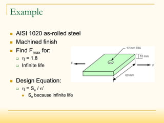
![Endurance limit modifying factors
Surface (ka)
Accounts for different surface finishes
Ground, machined, cold-drawn, hot-rolled, as-forged
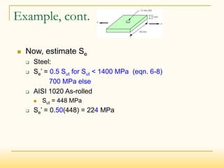
Size (kb)
Different factors depending on loading
Bending and torsion (see pg. 280)
Axial (kb = 1)
Loading (kc)
Endurance limits differ with Sut based on fatigue loading (bending, axial, torsion)
Temperature (kd)
Accounts for effects of operating temperature (Not significant factor for T<250 C [482 F])
Reliability (ke)
Accounts for scatter of data from actual test results (note ke=1 gives only a 50% reliability)
Miscellaneous-effects (kf)
Accounts for reduction in endurance limit due to all other effects
Reminder that these must be accounted for
Residual stresses
Corrosion
etc](https://image.slidesharecdn.com/7fatiqueload-210131073535/85/7-Machine-design-fatigue-load-22-320.jpg)
![Fatigue SC factor
kf = [1 + q(kt – 1)]
kfs = [1 + qshear(kts – 1)]
kt or kts and nominal stresses
Table A-15 & 16 (pages 1006-1013 in Appendix)
q and qshear
Notch sensitivity factor
Find using figures 6-20 and 6-21 in book (Shigley) for steels
and aluminums
Use q = 0.20 for cast iron
Brittle materials have low sensitivity to notches
As kf approaches kt, q increasing (sensitivity to notches, SC’s)
If kf ~ 1, insensitive (q = 0)
Property of the material](https://image.slidesharecdn.com/7fatiqueload-210131073535/85/7-Machine-design-fatigue-load-30-320.jpg)

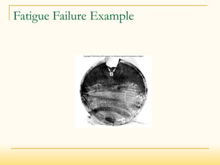
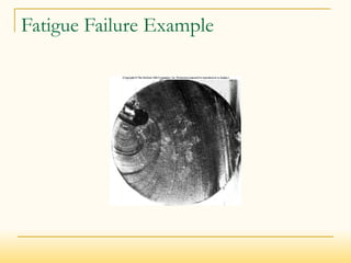
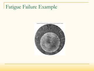
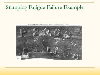
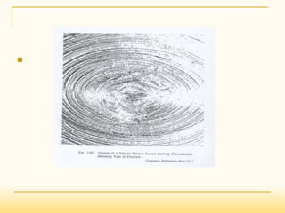
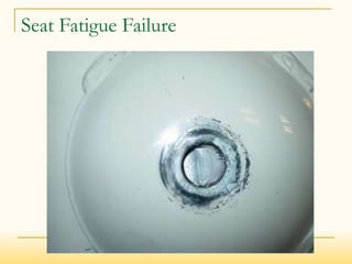
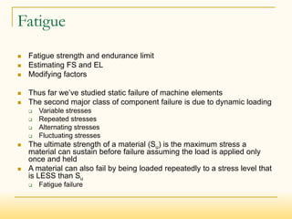
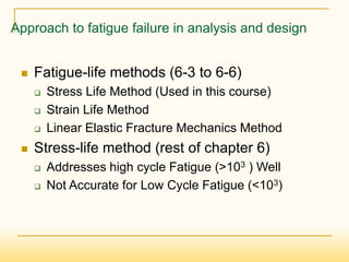
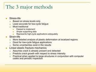
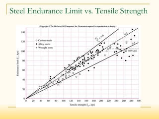
The document discusses fatigue failure and fatigue analysis. It begins by explaining that fatigue failure starts with a crack, usually at a stress concentration, which then propagates until sudden fracture. It then provides examples of fatigue failures and discusses different fatigue analysis methods. The key points are: - Fatigue failure results from repeated or fluctuating stresses that are lower than the material's ultimate strength. - It can be analyzed using stress-life, strain-life, or fracture mechanics methods, with stress-life most common for high-cycle fatigue. - The stress-life approach estimates fatigue strength (Sf) based on stress levels and uses modifying factors to account for real-world differences from test specimens.