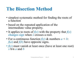
Chapter three focuses on root-finding techniques for nonlinear functions, emphasizing iterative methods to solve equations like f(x) = 0, which frequently occur in scientific applications. Key methods discussed include the bisection method, Newton-Raphson method, and secant method, with examples illustrating their implementation. The chapter also outlines the importance of numerical approximation for root finding, particularly in cases where analytical solutions are not feasible.

1. Chapter Three
Root Finding

2. Roots of Nonlinear Functions
• The most common real-life problems are nonlinear and
are not amenable to be handled by analytical methods to
obtain solutions of a variety of mathematical problems.
Iterative(reputation) methods are the foremost among the
methods developed to obtain approximate solutions.
• The method of finding a root of the non-linear
equations of the form
𝑓 𝑥 = 0
• where the function f(x) may be algebraic, transcendental
or combination of both, plays a major role in the
applications of mathematics as problems of such kind
occur more frequently in many scientific and
mathematical modeling.
Computational Physics Jifar R. 2

3. The following equations
i. 𝑥6– 𝑥 – 1 = 0
ii.𝑥𝑒𝑥
– cos 𝑥 = 0
iii.sin(𝑥)𝑒𝑥– 2𝑥 – 5 = 0
• can be classified as follows.
i.The equation 𝒙𝟔– 𝒙 – 𝟏 = 𝟎 is an algebraic equation of
degree 6 having one root nearly at x = 1.13472413.
ii.The equation 𝒙𝒆𝒙
– 𝒄𝒐𝒔 𝒙 = 𝟎 is a transcendental
equation as it contains transcendental functions which has
a root nearly about x = 0.51775736.
iii.The equation 𝒔𝒊𝒏(𝒙)𝒆𝒙– 𝟐𝒙 – 𝟓 = 𝟎 is an equation
combined of both algebraic and transcendental functions
and it has a root nearly about x = – 2.523245230.
Computational Physics Jifar R. 3

4. • If a number ‘𝜶’ makes the function of a scalar variable, i.e., 𝒇(𝒙) to
zero then ‘𝜶’ is called a zero or a root of the equation 𝒇(𝒙) = 𝟎.
• To obtain this root, if one obtains iterates {𝒙𝟏, 𝒙𝟐, … . 𝒙𝒏 … } starting
with an initial guess 𝑥0, then this sequence of iterates converge to the
root whenever
𝐥𝐢𝐦
𝒏→∞
𝒙𝒏 − 𝜶 = 𝟎 𝒐𝒓 𝐥𝐢𝐦
𝒏→∞
𝒙𝒏 = 𝜶
• In this chapter, we shall study the methods of obtaining
an approximate solution of equations of the form
𝑓 𝑥 = 0 and discuss the importance of each of these
methods comparing with one another when required,
through some examples.
Computational Physics Jifar R. 4

5. • Let f (x) be a real valued function defined for a ≤ x ≤ b.
• A number 𝑥0 is called a root of the function f (x) in this
interval if f (𝑥0) = 0 and, correspondingly, a number x
=𝑥0 that makes f (x) vanish is called a zero of f (x).
• The need to find roots of functions is fundamental to the
development and application in sciences
• Only in simple cases can the roots be determined
analytically, so in all other cases it is necessary to find
them numerically.
• Many different methods exist, of these only bisection
method, Secant method, & Newton’s method will be
described in any detail, as they are in everyday use and
are easily implemented on a computer.
Computational Physics Jifar R. 5

6. Roots of an equation
• In physics, we often encounter situations in which
we need to find the possible value of x that ensures
the equation f(x) = 0, where f(x) can either be an
explicit or an implicit function of x.
• If such a value exists, we call it a root or zero of the
equation
• In this section, we will discuss only single-variable
problems and leave the discussion of multivariable
cases to Chapter 5, after we have gained some basic
knowledge of matrix operations.
Computational Physics Jifar R. 6

7. The Bisection Method
• simplest systematic method for finding the roots of
a function
• based on the repeated application of the
intermediate value property.
• It applies to roots of f(x) with the property that f(x)
changes sign when x crosses a root.
• For a continuous function f(x) & numbers a < b:
f(a) and f(b) have opposite signs.
• f(x) must vanish at least once (have at least one root)
x b/n a and b
Computational Physics Jifar R. 7

8. Bisection Method
If a root exists in the region
method – simple method to code
for ,we can use the bisection
B/
c there is a root in the region,
We divide the region into two equal parts
Then we have either or
Roots of an Equation
a b
2
o
x =
a+b
x
f (x)
y
•
8
Computational Physics Jifar R.

9. Steps
1. Determine a & b
2. Bisect interval a ≤ x ≤ b into: a<x<x1 & x1<x<b,
x1 = 1/2(a + b) a x1 b
• If f(x1)= 0, then x1 is a root of f(x) = 0.
• Else
 the root lies b/n a & x1 or b/n x1 & b according as f(x1) is
+ve or –ve.
• If f(x1) > 0  x2 = (a + x1)/2
If f(x2)=0  x2 is root
• Else if f(x1) < 0  x3 = (b + x1)/2
If f(x3)=0  x3 is root
• Proceed the calculation until the first time successive iterates
xm and xm+1 satisfy the condition |xm − xm+1| < δ.
Computational Physics Jifar R. 9

10. Example
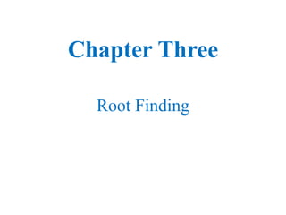
• Root of f(x) = 𝑥3
− 4x − 9 = 0, using the bisection
method correct to 3 decimal places
• Find [a,b] by trial that gives f(𝒂)<0 and f(𝒃)>0
• f(2) = – 9 <0 , f(3) = 6>0.  a=2, b=3.
2 x1 3
• This shows a root lies between 2 & 3.
• 𝑥1 =
1
2
a+b =
1
2
(2 + 3) = 2.5.
• f(x1) = -3.375 < 0  root is b/n x1 & 3, [2.5,3.0]
• 𝑥2 =
1
2
(𝑥1 + 3) = 2.75
• f(x2) = 0.7969 > 0  root is b/n x1 & x2, [2.5,2.75]
Computational Physics Jifar R. 10

11. Example
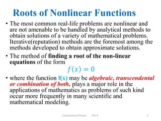
• 𝑥3 =
1
2
(𝑥1 + 𝑥2) = 2.625
• f(x3)=-1.4121< 0  root b/n x2 & x3, [2.75,2.625]
• 𝑥4 =
1
2
(𝑥2 + 𝑥3) = 2.6875,
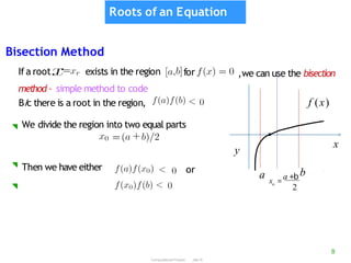
Repeating this process:
• x5=2.71875, x6=2.70313,
• x7=2.71094, x8=2.70703,
• x9= 2.70508, x10 = 2.70605,
• x11 = 2.70654, x12 = 2.70642
 The root is 2.70642
Computational Physics Jifar R. 11

12. Algorithm
1. Determine a & b
2. Bisect interval a ≤ x ≤ b into: a<x<x1 & x1<x<b,
x1 = 1/2(a + b)
a x1 b
3. Replace a by x1
If f(a) f(x1) > 0  f(x) changes sign in x1< x<b so this
interval contain root 𝑥𝑟.
If f(a) f(x1) < 0  replace b by x1, f(x) change sign in
α < x < x1, and so contain a root 𝑥𝑟
4. Proceed the calculation until the first time successive
iterates xm & xm+1 satisfy the condition |xm − xm+1| < δ.
Computational Physics Jifar R. 12

13. Program bisection
Implicit none
real :: x, a, b, x1, f, dx
integer :: itr, n, i
real, parameter :: del=10E-7 !del is the
error
a = 2.0 ; b = 3.0 ! a and b are the intervals
dx = b-a
n = int(log10(dx)-log10(del))/log10(2.0) + 1
do i = 1,n
x = (a+b)/2.0 !first mid value b/n a and b
if ( f(a)*f(x) < 0.0 )then !Checking starts
here
! if this is true then f(x)>0 b/c f(a)<0
b = x !x replaces b in x = (a+x)/2.0
else
!if f(a)*f(x)>0, this condition is true if
!f(x)<0 because f(a)<0.
a = x !x replaces a in x = (x+b)/2.0
End if
print*, x, f(x)
End do
print*,x
end program bisection
function f(x) ! used by program
implicit none
real::x, f
f = x**3 - 4.0*x - 9.0
end function f
Computational Physics Jifar R. 13

14. The Newton-Raphson method
• is based on linear approximation of a smooth function
around its root.
• Taylor expansion of 𝑓(𝑥𝑟) = 0 in the neighborhood of
𝑥𝑟
𝑓(𝑥𝑟) ≈ 𝑓(𝑥) + (𝑥𝑟 − 𝑥)𝑓′
(𝑥)+. . . = 0
• x is trial value for 𝑥𝑟 at 𝑘𝑡ℎ
step & approximate value of
the next step 𝑥𝑘+1 can be derived from:
𝑓(𝑥𝑘+1) = 𝑓(𝑥𝑘) + (𝑥𝑘+1 − 𝑥𝑘)𝑓′(𝑥𝑘) = 0,
that is,
𝒙𝒌+𝟏 = 𝒙𝒌 − 𝒇(𝒙𝒌) 𝒇′(𝒙𝒌)
• 𝑓′(𝑥𝑘) =
𝑑𝑓𝑘
𝑑𝑥
with k = 0, 1, . . . & 𝑓𝑘 = 𝑓(𝑥𝑘)
• The above iterative scheme is known as the Newton
method, or the Newton-Raphson method.
Computational Physics Jifar R. 14

15. Example: root of 𝑓(𝑥) = 𝑥3
− 4x − 9
• Use 𝑥0 =
𝑎+𝑏
2
= 2.5, from Bisection
• 𝑓𝑘
′
=
𝑑𝑓𝑘
𝑑𝑥
= 3𝑥𝑘
2
− 4
• 𝑥𝑘+1 = 𝑥𝑘 − 𝑓𝑘 𝑓𝑘
′
= 𝑥𝑘 −
𝑥𝑘
3−4x−9
3𝑥𝑘
2−4
• 𝑥𝑘+1 =
2𝑥𝑘
3+9
3𝑥𝑘
2−4
 𝑥1 =
2𝑥0
3+9
3𝑥0
2−4
=
2(2.5)3+9
3(2.5)2−4
= 2.7288136
 𝑥2 =
2𝑥1
3+9
3𝑥1
2−4
= 2.706749
Using the above
• x3 = 2.7065279
• x4 = 2.7065279 = 2.706528
• root is 2.706528, using Bisection it is 2.706482 almost the
same result, but Newton method converges faster
Computational Physics Jifar R. 15

16. The Secant Method
• when f(x) has an implicit dependence on x, df/dx
needed in Newton method may not exist or may be
very difficult to obtain.
• Alternative scheme to achieve a similar algorithm.
is to replace 𝑓𝑘 in the Newton method with the two-
point formula for df/dx,
𝑑𝑓(𝑥𝑘)
𝑑𝑥
=
𝑓(𝑥𝑘) − 𝑓(𝑥𝑘−1)
𝑥𝑘 − 𝑥𝑘−1
• Putting this in the Newton method:
𝒙𝒌+𝟏 = 𝒙𝒌 −
(𝒙𝒌 − 𝒙𝒌−𝟏)
𝒇𝒌 − 𝒇𝒌−𝟏
𝒇𝒌
Computational Physics Jifar R. 16

17. Example: root of 𝑓(𝑥) = 𝑥3
− 4x − 9
• Using 𝑓𝑘 = 𝑥𝑘
3
− 4𝑥k − 9 and
• initial values x0 = 2, x1=3,
• f0 = f(x0)= f(2)=-9, f1 = f(x1)=f(3)=6
• Then using 𝑥𝑘+1 = 𝑥𝑘 −
(𝑥𝑘−𝑥𝑘−1)
𝑓𝑘−𝑓𝑘−1
𝑓𝑘
• We are given 𝑥 at k=0 and k=1, find 𝑥 at 𝑘 ≥ 2
• 𝑥2 = 𝑥1 −
𝑥1−𝑥0
𝑓1−𝑓0
𝑓1 = 3 −
3−2
6+9
6 = 2.6, 𝑓2=𝑓(𝑥2) = −1.824
• 𝑥3 = 𝑥2 −
𝑥2−1
𝑓2−𝑓1
𝑓2 = 2.6 −
2.6−3
−1.824−6
(−1.824) = 2.693252
• Following the same trend for x4, x5, x6 and x7
• x7 = 2.706528 the same with newton method.
Computational Physics Jifar R. 17

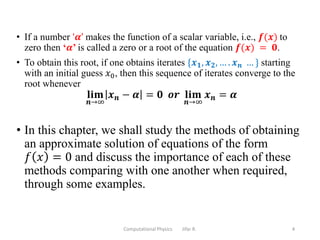
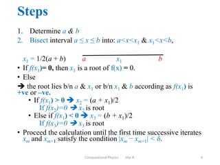
18. Exercise
Find the zeros of f 𝑥 = 1 − 3𝑥 +
1
2
𝑥𝑒𝑥 using
a) Bisection: use [0.43,0.47] and [1.53,1.57]
b) Newton: 𝑥0 = 0.5, and 𝑥0 = 1.6
c) Secant method: 𝑥0 = 0.43, 𝑥1 = 0.47
and 𝑥0 = 1.53, 𝑥1 = 1.57
To accurate to 5 decimal places. [two roots from the
graph can be shown]
Answer
𝑥4 =0.45154 1st root
𝑥4 =1.54954 2nd root
Computational Physics Jifar R. 18

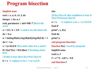
19. Assignment [3,4,5] 10%
For the following functions(1-3) use bisection, Newton-
Raphson & secant methods correct to 3 decimal places to
find their root and write f90 code that gives its root.
1) f(x) = 3x2 − 7x + 3 = 0
2) f(x) = 𝑥 − 𝑐𝑜𝑠𝑥 = 0
3) f(x) = 𝑥log𝑥 − 1.2 = 0, which lies between 2 and 3
4) Apply the secant method to solve f(x) = ex2
lnx2
− x = 0
5) Apply any of the three methods t find their root and
write f90 program for each.
a) xsin(x)+cos(x)
b) x3
− x2
− x + 1
c) cos(x) - x ex
Computational Physics Jifar R. 19