Behavioral Analysis of Second Order Sigma-Delta Modulator for Low frequency Applications

IOSR Journal of Computer Engineering (IOSR-JCE)
e-ISSN: 2278-0661, p- ISSN: 2278-8727Volume 10, Issue 1 (Mar. - Apr. 2013), PP 34-42
www.iosrjournals.org
www.iosrjournals.org 34 | Page
Behavioral Analysis of Second Order Sigma-Delta Modulator for
Low frequency Applications
Susmita S. Samanta1
, R.W. Jasutkar 2
1
(Department of Computer Science Engineering,G.H Raisoni College of Engineering,India)
2
(Department of Computer Science Engineering,G.H Raisoni College of Engineering,India)
Abstract: Switched capacitor (SC) based modulator is prone to various non-idealities; especially at the circuit
designing stage where the integrator plays an important role and effects the overall performance of the sigma
delta modulator. The non idealities take account of sampling jitter which includes the effect of switching
circuitry, sampling noise. Opamp parameter include noise, finite dc gain, finite band width, slew rate,
saturation voltage. Each non idealities is modeled mathematically and simulation is carried out in the
MATALAB SIMULINK®
environment with the help of sigma delta toolbox. The simulation analysis of each
model is carried out individually. At last overall performance of the modulator with all nonidealities is carried
out compared with the ideal modulator and satisfactory results were found out for second order sigma delta
modulator for signal bandwidth of 4 KHz.
Keywords: Sigma Delta modulator (∑Δ), Behavioral Analysis, Switch Capacitor (SC),Genetic Algorithm(GA).
I. INTRODUCTION
Sigma delta modulator are exploited in various applications like wireless communication devices,
consumer electronics, biomedical applications. The oversampling property of the sigma delta modulator employ
coarse quantization enclosed in one or more feedback loops. By sampling at a frequency much higher than the
signal bandwidth it is possible for the feedback loops to shape the quantization noise so that most of the noise
power is shifted out of the signal band [1]. This is illustrated in fig.1
Fig.1 Low frequency noise is pushed to high frequencies by noise shaping
The out of band noise can then be attenuated with a digital filter. The degree to which the quantization noise can
be attenuated depends on the order of the noise shaping and oversampling ratio. Sigma delta modulators are
suitable for low frequency, high resolution applications, in keeping view of their linearity property, reduced
requirement of the antialiasing filter, and its robustness. ∑Δ modulator allows high performance to achieve
without effecting accuracy and speed with low sensitivity to analog component imperfections or component
trimming.
ΣΔ modulators can be implemented either with continuous-time or with discrete-data techniques. The
most popular approach is based on a discrete-data solution with switched capacitor (SC) implementation. As the
technology is scaling down into a deep submicron level transistor sizing has become an issue. The fact that,SC
ΣΔ modulators can be effectively realized in standard CMOS technology without any performance degradation.
During the design phase of an SDM the noise-shaping transfer function is typically evaluated using a linear
model. For a 1-bit quantizer, the noise transfer is highly non-linear and large differences between predicted and
actual realized transfer can occur. The linear modeling is used to evaluate the performance of the sigma delta
modulator through simulation [2]. Various criteria exits to evaluate the performance of the SMD.

Behavioral Analysis of Second Order Sigma-Delta Modulator for Low frequency Applications
In practice, a significant problem in the design of the sigma delta modulators is the estimation of their
performance, science they are mixed signal non linear circuits. Due to the nonlinearity of the modulator loop the
optimization of the performance has to be carried out with behavioral time domain analysis. For high
performance accurate simulation of number of non idealities and eventually, comparison of performance of
different architecture are needed in order to choose the best possible solution. A large set of parameters need to
optimize so as to achieve the desired signal to noise ratio (SNR). Therefore, in this paper we present a complete
set of SIMULINK models, which allow us to perform exhaustive time-domain behavioral analysis of any ΣΔ
modulator taking into account most of the non-idealities, such as sampling jitter, kT/C noise and operational
amplifier parameters (noise, finite dc gain, finite bandwidth, slew-rate (SR) and saturation voltages).The
following sections describe in detail each of the models presented. Finally, simulation results, which
demonstrate the validity of the models proposed, are provided. All the simulations were carried out on 2nd-order
SC ΣΔ modulator architecture.
Fig. 2 Block diagram of 2nd
order ΣΔ modulator
II. NON-IDEALITIES IN SMD
The block diagram of second order sigma delta modulator is shown in Fig.2 .The modulator consist of
input sampler, an integrator, a quantizer/comparator and feedback loop which consist of a digital to analog
converter (DAC).Depending upon the number of the integrator the order of the modulator is decided. The
integrator integrates the input signal over on each clock cycle, which operates a much higher frequency than the
sampling frequency. This property of oversampling is being exploited in the sigma delta modulator. The
integration of the pulse difference is linear over one clock cycle. The output of the integrator is then fed to the
quantizer. The quantizer then digitized the input signal. The feedback path shifts the logic level of the input, so
that it matches the logic level of the input.
The schematic of a first-order SC ΣΔ modulator is shown in Fig.3. The main nonidealities appearing in the
SC circuitry, which should be considered for accurate modeling, are as follows:
 Clock jitter
 Switch thermal noise
 Operational amplifier noise
 Opamp DC gain
 Opamp Bandwidth(BW)
 Opamp slew rate(SR)
They will be thoroughly discussed in the following sections. The simulation environment will be done on the
output samples in the time domain. The nonidealities mentioned above produce a deviation of the output
samples from their ideal values.
Fig. 3 Schematic of first order ΣΔ modulator
III. CLOCK JITTER
The clock jitter is sometimes referred as sampling jitter as it is determined by computing the effects on
sampling the input signal. The jitter noise induced by the clock of is independent of the system architecture
[4].The effect of sampling jitter on SC Sigma delta modulator can be calculated easily, since the operation of the

SC depends on complete switching of the charge during each of the clock phase [5]. In fact, once the analog
signal has been sampled, the SC circuit is a sampled data system where variations of the clock period have no
direct effect on the circuit performance. Therefore, the effect of clock jitter on an SC circuit is completely
described by computing its effect on the sampling of the input signal.
The clock jitter results in a non-uniform sampling time sequence and thus increases the total error
power in the quantizer output. The magnitude of this error is a function of the statistical properties of the jitter
and the input signal to the system. When the input is a sinusoidal, the error introduced by jitter can be modeled
by
𝑥 𝑡 + 𝛿 − 𝑥 𝑡 ≈ 2𝜋𝑓𝑖𝑛 𝛿𝐴 cos 2𝜋 𝑓𝑖𝑛 𝑡 =
𝛿𝑑𝑥 (𝑡)
𝑑𝑡
(1)
The input sinusoidal signal is 𝑥 𝑡 , A is the amplitude of the signal. Frequency 𝑓𝑖𝑛 is sampled at an instant which
is in error by an amount 𝛿 is given Eqn. (1). The input signal x(t) and its derivative (du / dt) are continuous-time
signals. They are sampled with sampling period TS by a zero order hold. Here, we assumed that the sampling
uncertainty 𝛿 is a Gaussian random process n(t) with standard deviation ∆𝜏. The signal n(t) is implemented
starting from a sequence of random numbers with Gaussian distribution, zero mean, and unity standard
deviation. Whether oversampling is helpful in reducing the error introduced by the jitter depends on the nature
of the jitter. Since we assume the jitter white, the resultant error has uniform power-spectral density (PSD) from
0 to fs /2. This effect can be simulated with SIMULINK®
by using the model shown in Fig.4, which implements
Eqn. (1).
Fig.4 SIMULINK model for random clock jitter
IV. NOISE ON INTEGRATOR
The most dominant noise sources affecting the operation of a switch capacitor of SMD are the
resistance of the switches in the on state and the amplifier [6]. The total noise power of the circuit is the sum of
the theoretical loop quantization noise power, the switch noise power and the op-amp noise power. These effects
can be simulated with SIMULINK using “noisy” integrator model shown in Fig. 5. The variable 𝑎 =
𝐶𝑠
𝐶𝑟
represents the integrator coefficient. The noise source like switches thermal noise and operational
amplifier noise and its relevant model is described in the following sub-sections.
Fig. 5 “Noisy” Integrator Model
A. Switches Thermal Noise
The thermal noise associated to the sampling switches and the intrinsic noise of the operational
amplifiers effects the operation of the modulator. According to Nyquist theorem the spectral density of noise at
the terminals of a dipole passive depends only on the temperature and the real part of impedance of the dipole.

In a switched capacitor integrator switches operate in ohmic region, the noise power at their terminals is equal
to:
𝐸𝑠𝑓𝑓
2
= 𝛾 𝑓 ∆𝑓 = 4𝐾𝑇𝑅∆𝑓 (2)
The noise due to switch on phases I and P is given by the Eqn. (3) and (4) respectively:
𝑉𝑡𝑕𝑃
2
=
𝐾𝑇
𝐶 𝑠
+
𝐶 𝑟.𝐾𝑇
2
𝐶 𝑠
2.𝐶 𝑟
(3)
𝑉𝑡𝑕𝐼
2
=
𝐾𝑇
𝐶 𝑠
+
𝐾𝑇
𝐶 𝑟
(4)
K is the Boltzmann constant and T the absolute temperature in Kelvin. The equations (3) and (4) show that if we
wishes to reduce the thermal noise power, then we must increase the
Fig. 6 Model of switches thermal noise
value of the sampling capacity Cs [7]. Thus the total noise can be evaluated by the following equation:
𝑒 𝑇
2
=
𝐾𝑇
𝐶 𝑠
(5)
The switch thermal noise voltage eT (usually called kT/C noise) is then superimposed to the input voltage x(t)
leading to:
𝑦 𝑜𝑢𝑡 = 𝑥 𝑡 + 𝑒𝑡 𝑡 𝑏 = 𝑥 𝑡 +
𝐾𝑇
𝐶 𝑠
𝑛(𝑡) 𝑏 (6)
where 𝑛(𝑡) denotes a Gaussian random process with unity standard deviation, while 𝑏 is the integrator gain Eqn.
6 is implemented by the model shown in Fig. 6.
B. Operational Amplifier Noise
The sources of noise present in an amplifier are generally two reasons for the thermal noise and noise
in 1/ f . For a MOS transistor in saturation, the voltage generator noise equivalent to the two sources is given by
[7]:
𝑆 𝐸𝑛 ≈ 22
3
𝐾𝑇.𝑔 𝑚
−1 +
𝐾 𝑓
𝐶 𝑜𝑥 𝑊𝐿
.
1
𝑓
(7)
Fig. 7 shows the model used to simulate the effect of the operational amplifier noise.
Fig.7 SIMULINK model of Operational Amplifier Noise
Here, Vn represents the total rms noise voltage referred to the op-amp input. Flicker (1/f) noise, wide-band
thermal noise and the dc offset contribute to this value. The total op-amp noise power (Vn)2
can be evaluated,
through circuit simulation, on the circuit of Fig. 2 during phase Φ2, by adding the noise contributions of all the
devices referred to the op-amp input and integrating the resulting value over the whole frequency spectrum.

V. NONIDEALITIES OF INTEGRATOR
Analog circuit implementations of the integrator deviate from this ideal behavior due to several non-
ideal effects. One of the major causes of performance degradation in SC ΣΔ modulators, indeed, is due to
incomplete transfer of charge in the SC integrators. This non-ideal effect is a consequence of the op-amp non-
idealities, namely finite gain and BW, slew rate (SR) and saturation voltages. These will be considered
separately in the following subsections. Fig. 8 shows the model of the real integrator including all the non-
idealities.
Fig.8 Real Integrator model
A. DC Gain
The DC gain of the ideal integrator is infinite. In practice, the gain of the operational amplifier open
loop A0 is finite. This is reflected by the fact that a fraction of the previous. Sample out of the integrator is added
to the sample input [8]. The model of a real integrator with an integrator delay is real considering the saturation
op-amp, the gain over the finite bandwidth and slew-rate. The Z transfer function of a perfect integrator is given
by:
𝐻 𝑧 =
𝑍−1
1−𝑍−1 (8)
The transfer function of the real integrator becomes:
𝐻 𝑧 = 𝛽
𝑍−1
1−𝛼𝑍 −1 (9)
where α and β are the integrator’s gain and leakage, respectively [9].
∝ =
𝐴0−1
𝐴0
(10)
The limited gain at low frequencies increases the in-band noise.
B. Bandwidth and SR
The distortion limits the power effectively used by the system and its bandwidth. There are various
reasons why a signal distorts. Regarding the harmonic distortion, it is mainly due to two factors of nonlinearity
and slew-rate of the amplifiers
a) Nonlinearity of the amplifiers
Theoretically its transfer function is:
𝑉𝑠 = 𝐴. 𝑉𝑒 (11)
A is the amplification factor whose transfer function is approximated given by (12) [10].
𝐴 ≅ 1 +∝1 𝑉0 +∝2 𝑉0
2
+ ∝3 𝑉0
3
+ … . (12)
Where (∝1,∝2, ∝3, … ) are the amplification factors parasites. Thus, for a pure sinusoidal signal of frequency f
in the input of the amplifier, we find the output of the amplifier, amplify the output signal with other parasitic
elements and proportional to the frequency fr , in this case we say that there is harmonic distortion, because this
spectrum of frequencies 2 f , 3 f , etc... .The total harmonic distortion is the ratio of the sum of squared
amplitudes of these signals on the amplitude of the fundamental.
b) Amplifier Slew Rate
For given constant amplitude, slew-rate characterizes the limit of the amplifier frequency (maximal
speed). When a signal is changing more slowly than the maximal speed, the amplifier follows and reproduces
faithfully the signal. But when the signal frequency increases (for constant amplitude), the amplifier distorts the
output signal. In this case, in addition to the original signal, there are additional frequencies (harmonics). The

augmentation of the input signal frequency creates difficulty to the amplifier to restore the signal faithfully. For
the amplifier responds linearly, it generally we define a maximum frequency above which the amplifier distorts
the output signal. For a sinusoidal signal of amplitude A pulsation ω , this frequency is defined by
𝐺𝐵𝑊 = 2𝜋𝐴𝑓 ≤ 𝑆𝑅 𝑓 =
𝑆𝑅
2𝜋𝐴
(13)
For a converter it is:
𝑓 =
1
2𝜋𝐴2 𝑛 𝜏
(14)
T is the settling time, τ = 1/ 2πGBW and n the resolution of the converter. In the case of a switched-capacitor
integrator (the main constituent of a 𝛴𝛥 modulator) the maximum speed cause an error "settling error" on the
output voltage of the integrator. Indeed, the finite width of the band and "slew-rate" of the amplifier are related
and may occur in the switched-capacitor circuit transient response non-ideal operation, "slew-rate" producing
each clock tick an incomplete charge transfer at the end of the integration period. The effect of the finite
bandwidth and the slew-rate are related to each other and may be interpreted as a non-linear gain.
Fig. 9 SIMULINK model of second–order ΣΔ modulator
VI. SIMULATION RESULTS
To validate the proposed model designed for various non-idealities, we perform various simulations on
the SIMULINK model on the model shown in Fig.9. A minimum SNDR of 90dB is required for the low
frequency biomedical applications. The simulation parameters used for simulation are summarized in Table I.
Table II compares the total SNDR and the corresponding effective number of bits (ENOB) which is nothing but
the maximum number of resolution can be obtained from the architecture.
TABLE I
SIMULATION PARAMETERS
Parameter Value
Signal Bandwidth BW = 4Khz
Sampling frequency
Oversampling Ratio
Sampling number
Integrator Gain
Fs = 1.008MHz
R = 126
N = 16384
b1 = b2 = 0.5
TABLE II
SIMULATION RESULTS
2nd
order ΣΔ
Modulator
Parameter
SNDR
[dB]
ENOB
[bits]
Ideal 101.5 16.56
Sampling jitter
(Δτ = 6ns)
90.7 14.77
Switches ( kT/C)
noise (Cs= 6pF)
89.5 14.58
Finite bandwidth
(GBW = 8.6MHz)
92.4 15.05
Slew Rate
(SR = 16V/µs)
90.4 14.72
Saturation Voltages
(𝑉𝑚𝑎𝑥 = ±5𝑉)
89.4 14.56

(a)
(b)
(C)
(d)

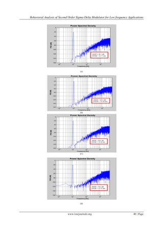
(e)
Fig. 10. PSD of (a) Sampling jitter Δτ = 6ns (b) Switches ( kT/C) noise Cs= 6pF (c)GBW = 8.6MHz(d) Slew Rate SR = 16V/µs
(e) Saturation Voltage 𝑉𝑚𝑎𝑥 = ±5𝑉)
Fig. 11.Comparison plot of the Ideal SMD and SMD with Non Idealities
VII. CONCLUSION
In this paper a modeling of second order sigma delta modulator is studied with various nonidealities of
the modulator like operational amplifier noise, thermal noise, finite DC gain and comparison of ideal and non
ideal SMD has also been done. The experimental results show that, SMD which is presented here have
similarity with the ideal modulator. The performance of the second order ΣΔ modulator can be further being
improved with the help of evolutionary algorithms like genetic algorithm (GA). Future work can be done with
modeling of the SMD with GA.
REFERENCES
[1] Dragi.a Milovanović , Milan Savić , Miljan Nikolić, “Second-Order Sigma-Delta Modulator in Standard CMOS Technology”,
SERBIAN JOURNAL OF ELECTRICAL ENGINEERING Vol. 1, No. 3, November 2004, 37 – 44
[2] E. Janssen, A. van Roermund, “Look-Ahead Based Sigma-Delta Modulation”, Analog Circuits and Signal Processing, DOI
10.1007/978-94-007-1387-1_2, © Springer Science+Business Media B.V. 2011
[3] Shashant Jaykar, Prachi Palsodkar, Pravin Dakhole, “Modeling of Sigma-Delta Modulator Non-Idealities in MATLAB/SIMULINK”,
2011 International Conference on Communication Systems and NetworkTechnologies, 978-0-7695-4437-3/11 $26.00 © 2011 IEEE
DOI 10.1109/CSNT.2011.112
[4] E. Farshidi, S. M. Sayedi, “A Second-order Low Power Current- Mode Continuous-Time Sigma-Delta Modulator,” ASICON'07,
Proceeding of the 7th IEEE International Conference on ASIC, Guilin, China, pp.293- 296, Oct. 2007
[5] E. Boser and B. A. Wooley, “The Design of Sigma-Delta Modulation Analog-to-Digital Converters”, IEEE J. Solid- State Circ., vol.
23, pp. 1298-1308, Dec. 1988.
[6] S. Brigati, F. Francesconi, P. Malcovati, D. Tonietto, A. Baschirotto and F. Maloberti, “MODELING SIGMA-DELTA
MODULATOR NONIDEALITIES IN SIMULINK®,” IEEE International Symposium, pp 384 - 387 vol.2, 1999.
[7] Abdelghani Dendouga , Nour-Eddine Bouguechal, Souhil Kouda and Samir Barra, “Modeling of a Second Order Non-Ideal Sigma-
Delta Modulator”, International Journal of Electrical and Compute Engineering 5:6 2010
[8] G. Temes, “Finite amplifier gain and bandwidth effects in switched capacitor filters,” IEEE J. Solid-State Circuits, vol. 15, pp.
358361, June1980.
[9] H. Zare-Hoseini and I. Kale, “On the effects of finite and nonlinear DCgain on the switched-capacitor delta-sigma modulators,” in
Proc. IEEE Int. Symp. Circuits Systems, May 2005, pp. 2547–2550.

[10] F. Medeiro et al., “Modeling opamp-induced harmonic distortion for switched-capacitor SD modulator design,” in IEEE Int. Symp.
Circuits Systems, vol. 5, May-Jun. 1994, pp. 445–448.
[11] Ms.R.W.Jasutkar, Dr.P.R.Baja,j Dr.A.Y.Deshmukh, “GA Based Low Power Sigma Delta Modulator for Biomedical Applications”,
978-1- 4244-9477-4/11/$26.00 ©2011 IEEE
[12] Youngcheol Chae and Gunhee Han “A Low Power Sigma Delta Modulator Using Class-C Inverter” in 2007 Symposium on VLSI
circuits Digest of Technical Papers.
[13] Shanthi Pavan, and Prabu Sankar “Power Reduction in Continuous-Time Delta-Sigma Modulators Using the Assisted Opamp
Technique” in IEEE Journal Of Solid-State Circuits, Vol. 45, No. 7, July 2010.
[14] Arnold R. Feldman, Bernhard E. Boser, and Paul R. Gray, Fellow, “A 13-Bit, 1.4-MS/s Sigma–Delta Modulator for RF Baseband
Channel Applications” in IEEE Journal Of Solid-State Circuits, Vol. 33, No. 10, October 1998.
[15] M.Loulou, D.Dallet and P.Marchegay “A 3.3V Switched Current Second Order Sigma Delta Modulator for Audio Applications” in
IEEE 2000.
[16] Ebrahim Farshidi, Navid Alaei-Sheini “A Micropower Current Mode Sigma Delta Modulator for Biomedical Applications” in IEEE
2009.
[17] Chen Yueyang, Zhong Shun’an, Dang Hua “Design of A low-power consumption and high-performance sigma-delta Modulator” in
2009World Congress on Computer Science and Information Engineering 978-0-7695-3507-4/08 $25.00 © 2008 IEEE.
[18] Guo-Ming Sung, Chih-Ping Yu, Dong-An Yao “A Comparison of Second-Order Sigma-Delta Modulator Between Switched-
Capacitor and Switched-Current Techniques” in 978-1-4244-2342-2/08/$25.00 ©2008 IEEE.

Behavioral Analysis of Second Order Sigma-Delta Modulator for Low frequency Applications

More Related Content

What's hot

Viewers also liked

Similar to Behavioral Analysis of Second Order Sigma-Delta Modulator for Low frequency Applications

More from IOSR Journals

Recently uploaded

Behavioral Analysis of Second Order Sigma-Delta Modulator for Low frequency Applications