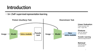
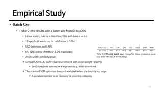
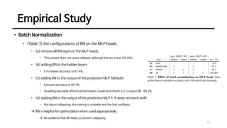
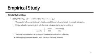
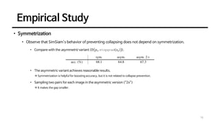
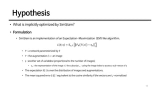
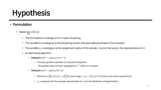
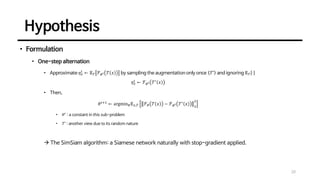
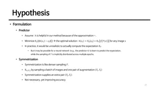
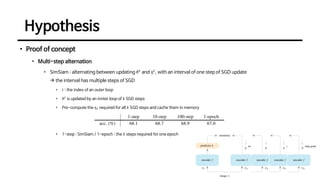
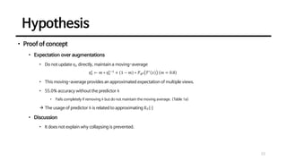
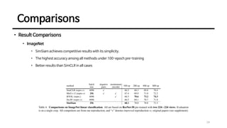
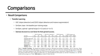
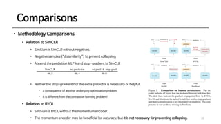
Sungchul Kim
Contents
1. Introduction
2. Method
3. Empirical Study
4. Comparisons
5. (Hypothesis)
2
Introduction
3
• Un-/Self-supervised representation learning
Pretext (Auxiliary) Task
Image Model Extra module
Pseudo
-task
Downstream Task
Image Model
New
extra module
Linear Evaluation
Freeze extractor and
train 1-layer NN
Finetune
Train all networks
for downstream
Transfer Learning
Detection/segmentation
Retrieval
Calculate Recall
among kNN
Introduction
4
• Siamese networks
• An undesired trivial solution : all outputs “collapsing” to a constant
• Constrastive Learning
• Attract the positive sample pairs and repulse the negative sample pairs
• SimCLR, MoCo, …
• Clustering
• Alternate between clustering the representations and learning to predict the cluster assignment
• SwAV
• BYOL
• A Siamese network in which one branch is a momentum encoder
Introduction
5
• SimSiam
• Without the momentum encoder, negative pairs, and online clustering
• Does not cause collapsing and can perform competitively
• Siamese networks : inductive biases for modeling invariance
• Invariance : two observations of the same concept should produce the same outputs.
• The weight-sharing Siamese networks can model invariance w.r.t. more complicated transformations
(augmentations).
Method
6
• SimSiam
• Two randomly augmented views 𝑥1 and 𝑥2 from an image 𝑥
• An encoder network 𝑓 consisting of a backbone and a projection MLP head
• Two output vectors 𝑝1 ≜ ℎ 𝑓 𝑥1 and 𝑧2 ≜ 𝑓 𝑥2
𝒟 𝑝1, 𝑧2 = −
𝑝1
𝑝1 2
⋅
𝑧2
𝑧2 2
• A symmetrized loss
ℒ =
1
2
𝒟 𝑝1, 𝑧2 +
1
2
𝒟 𝑝2, 𝑧1
• Stop-gradient operation
ℒ =
1
2
𝒟 𝑝1, stopgrad 𝑧2 +
1
2
𝒟 𝑝2, stopgrad 𝑧1
Method
7
• SimSiam
• Baseline Settings
• Optimizer
• SGD with 0.9 momentum and weight decay 0.0001
• Learning rate : 𝑙𝑟 × BatchSize/256 with a base 𝑙𝑟 = 0.05
• Batch size : 512 / Batch normalization synchronized across devices
• Projection MLP
• (FC (2048) + BN + ReLU) x 2 + FC (𝑑=2048) + BN (𝑧)
• Prediction MLP
• FC (512)+ BN + ReLU + FC (𝑑=2048) (𝑝)
• Experimental setup
• Pre-training : 1000-class ImageNet training set
• Linear evaluation : training a supervised linear classifier on frozen representations
Empirical Study
8
• Stop-gradient
• (Left) quickly find a degenerated solution reach the minimum possible loss of -1 without stop-gradient
• (middle) std of the 𝑙2-normalized output z′
= 𝑧/ 𝑧 2
• The outputs collapse to a constant vector → the std over all samples should be zero for each channel! (the red curve)
• The output 𝑧 has a zero-mean isotropic Gaussian distribution → the std of 𝒛′ is
𝟏
𝒅
→ The outputs do not collapse, and they are scattered on the unit hypersphere!
• 𝑧𝑖
′
= Τ
𝑧𝑖 σ𝑗=1
𝑑
𝑧𝑗
2
1
2
≈ Τ
𝑧𝑖 𝑑
1
2 (if 𝑧𝑗 is subject to an i.i.d Gaussian distribution) → std 𝑧𝑖
′
≈ 1/𝑑
1
2
Empirical Study
9
• Stop-gradient
• (Right) the validation accuracy of a k-nearest-neighbor (kNN) classifier
• The kNN classifier can serve as a monitor of the progress.
• With stop-gradient, the kNN monitor shows a steadily improving accuracy!
• (Table) the linear evaluation result
• w/ stop-grad : a nontrivial accuracy of 67.7%
• w/o stop-grad : 0.1%..
Empirical Study
10
• Stop-gradient
• Discussion
• There exist collapsing solutions.
• The minimum possible loss and the constant outputs (Of course, it is not sufficient to indicate collapsing!)
• It is insufficient for our method to prevent collapsing solely by the architecture designs (e.g., predictor, BN, 𝑙2-norm).
Empirical Study
11
• Predictor
• (Table 1) the predictor MLP (ℎ)’s effect
• (a) removing ℎ (=ℎ is the identity mapping) → the model does not work!
• ℒ(a) =
1
2
𝒟 𝑧1, stopgrad 𝑧2 +
1
2
𝒟 𝑧2, stopgrad 𝑧1
• Same direction as the gradient of 𝒟 𝑧1, 𝑧2 with the magnitude scaled by 1/2 → collapsing!
• The asymmetric variant 𝒟 𝑝1, stopgrad 𝑧2 also fails if removing ℎ, while it can work if ℎ is kept.
Empirical Study
12
• Predictor
• (Table 1) the predictor MLP (ℎ)’s effect
• (b) ℎ is fixed as random initialization → the model does not work!
• This failure is not about collapsing. The training does not converge, and the loss remains high.
• (c) ℎ with a constant 𝑙𝑟 (without decay) → works well!
• It is not necessary to force it converge (by reducing 𝑙𝑟) before the representations are sufficiently trained.
Empirical Study
13
• Batch Size
• (Table 2) the results with a batch size from 64 to 4096
• Linear scaling rule (𝑙𝑟 × BatchSize/256) with base 𝑙𝑟 = 0.5
• 10 epochs of warm-up for batch sizes ≥ 1024
• SGD optimizer, not LARS
• 64, 128 : a drop of 0.8% or 2.0% in accuracy
• 256 to 2048 : similarly good
→ SimSiam, SimCLR, SwAV : Siamese network with direct weight-sharing
→ SimCLR and SwAV both require a large batch (e.g., 4096) to work well.
→ The standard SGD optimizer does not work well when the batch is too large.
→ A specialized optimizer is not necessary for preventing collapsing.
Empirical Study
14
• Batch Normalization
• (Table 3) the configurations of BN on the MLP heads
• (a) remove all BN layers in the MLP heads
• This variant does not cause collapse, although the acc is low (34.6%).
• (b) adding BN to the hidden layers
• It increases accuracy to 67.4%.
• (c) adding BN to the output of the projection MLP (default)
• It boosts accuracy to 68.1%.
• Disabling learnable affine transformation (scale and offset) in 𝑓’s output BN : 68.2%
• (d) adding BN to the output of the prediction MLP ℎ → does not work well!
• Not about collapsing, the training is unstable and the loss oscillates.
→ BN is helpful for optimization when used appropriately.
→ No evidence that BN helps to prevent collapsing.
Empirical Study
15
• Similarity Function
• Modify 𝒟 as: 𝒟 𝑝1, 𝑧2 = −softmax 𝑧2 ⋅ log softmax 𝑝1
• The output of softmax can be thought of as the probabilities of belonging to each of 𝑑 pseudo-categories.
• Simply replace the cosine similarity with the cross-entropy similarity, and symmetrize it.
• The cross-entropy variant can converge to a reasonable result without collapsing.
→ The collapsing prevention behavior is not just about the cosine similarity.
Empirical Study
16
• Symmetrization
• Observe that SimSiam’s behavior of preventing collapsing does not depend on symmetrization.
• Compare with the asymmetric variant (𝒟 𝑝1, stopgrad 𝑧2 ).
• The asymmetric variant achieves reasonable results.
→ Symmetrization is helpful for boosting accuracy, but it is not related to collapse prevention.
• Sampling two pairs for each image in the asymmetric version (“2x”)
→ It makes the gap smaller.
Empirical Study
17
• Summary
• SimSiam can produce meaningful results without collapsing.
• The optimizer (batch size), batch normalization, similarity function, and symmetrization
→ affect accuracy, but we have seen no evidence about collapsing prevention
→ the stop-gradient operation may play an essential role!
Hypothesis
18
• What is implicitly optimized by SimSiam?
• Formulation
• SimSiam is an implementation of an Expectation-Maximization (EM) like algorithm.
ℒ 𝜃, 𝜂 = 𝔼𝑥,𝒯 ℱ𝜃 𝒯 𝑥 − 𝜂𝑥 2
2
• ℱ : a network parameterized by 𝜃
• 𝒯 : the augmentation / 𝑥 : an image
• 𝜂 : another set of variables (proportional to the number of images)
• 𝜂𝑥 : the representation of the image 𝑥 / the subscript 𝑥 : using the image index to access a sub-vector of 𝜂
• The expectation 𝔼 ⋅ is over the distribution of images and augmentations.
• The mean squared error ⋅ 2
2
: equivalent to the cosine similarity if the vectors are 𝑙2-normalized
Hypothesis
19
• Formulation
• Solve min
𝜃,𝜂
ℒ 𝜃, 𝜂
• This formulation is analogous to k-means clustering.
• The variable 𝜃 is analogous to the clustering centers (the learnable parameters of an encoder)
• The variable 𝜂𝑥 is analogous to the assignment vector of the sample 𝑥 (a one-hot vector, the representation of 𝑥)
• An alternating algorithm
• Solving for 𝜽 (𝜃𝑡
← argmin𝜃ℒ 𝜃, 𝜂𝑡−1
)
• The stop-gradient operation is a natural consequence
: the gradient does not back-propagate to 𝜂𝑡−1
which is a constant.
• Solving for 𝜼 (𝜂𝑡
← argmin𝜂ℒ 𝜃𝑡
, 𝜂 )
• Minimize 𝔼𝒯 ℱ𝜃𝑡 𝒯 𝑥 − 𝜂𝑥 2
2
for each image 𝑥 : 𝜂𝑥
𝑡
← 𝔼𝒯 ℱ𝜃𝑡 𝒯 𝑥 (due to the mean squared error)
• 𝜂𝑥 is assigned with the average representation of 𝑥 over the distribution of augmentation.
Hypothesis
20
• Formulation
• One-step alternation
• Approximate 𝜂𝑥
𝑡
← 𝔼𝒯 ℱ𝜃𝑡 𝒯 𝑥 by sampling the augmentation only once (𝒯′) and ignoring 𝔼𝒯 ⋅
𝜂𝑥
𝑡
← ℱ𝜃𝑡 𝒯′
𝑥
• Then,
𝜃𝑡+1
← argmin𝜃𝔼𝑥,𝒯 ℱ𝜃 𝒯 𝑥 − ℱ𝜃𝑡 𝒯′
𝑥 2
2
• 𝜃𝑡
: a constant in this sub-problem
• 𝒯′ : another view due to its random nature
→ The SimSiam algorithm: a Siamese network naturally with stop-gradient applied.
Hypothesis
21
• Formulation
• Predictor
• Assume : ℎ is helpful in our method because of the approximation ~.
• Minimize 𝔼𝑧 ℎ 𝑧1 − 𝑧2 2
2
→ the optimal solution : ℎ 𝑧1 = 𝔼𝑧 𝑧2 = 𝔼𝒯 𝑓 𝒯 𝑥 for any image 𝑥
• In practice, it would be unrealistic to actually compute the expectation 𝔼𝒯
• But it may be possible for a neural network (e.g., the predictor ℎ) to learn to predict the expectation,
while the sampling of 𝒯 is implicitly distributed across multiple epochs.
• Symmetrization
• Symmetrization is like denser sampling 𝒯.
• 𝔼𝑥,𝒯 ⋅ by sampling a batch of images and one pair of augmentation 𝒯
1, 𝒯
2
• Symmetrization supplies an extra pair 𝒯
2, 𝒯
1
• Not necessary, yet improving accuracy
Hypothesis
22
• Proof of concept
• Multi-step alternation
• SimSiam : alternating between updating 𝜃𝑡
and 𝜂𝑡
, with an interval of one step of SGD update
→ the interval has multiple steps of SGD
• 𝑡 : the index of an outer loop
• 𝜃𝑡
is updated by an innter loop of 𝑘 SGD steps
• Pre-compute the 𝜂𝑥 required for all 𝑘 SGD steps and cache them in memory
• 1-step : SimSiam / 1-epoch : the 𝑘 steps required for one epoch
Hypothesis
23
• Proof of concept
• Expectation over augmentations
• Do not update 𝜂𝑥 directly, maintain a moving-average
𝜂𝑥
𝑡
← 𝑚 ∗ 𝜂𝑥
𝑡−1
+ 1 − 𝑚 ∗ ℱ𝜃𝑡 𝒯′
𝑥 𝑚 = 0.8
• This moving-average provides an approximated expectation of multiple views.
• 55.0% accuracy without the predictor ℎ
• Fails completely if removing ℎ but do not maintain the moving average. (Table 1a)
→ The usage of predictor ℎ is related to approximating 𝔼𝒯 ⋅
• Discussion
• It does not explain why collapsing is prevented.
Comparisons
24
• Result Comparisons
• ImageNet
• SimSiam achieves competitive results with its simplicity.
• The highest accuracy among all methods under 100-epoch pre-training
• Better results than SimCLR in all cases
Comparisons
25
• Result Comparisons
• Transfer Learning
• VOC (object detection) and COCO (object detection and instance segmentation)
• SimSiam, base : the baseline pre-training recipe
• SimSiam, optimal : optimal recipe (𝑙𝑟=0.5 and 𝑤𝑑=1e-5)
• Siamese structure is a core factor for their general success.
Comparisons
26
• Methodology Comparisons
• Relation to SimCLR
• SimSiam is SimCLR without negatives.
• Negative samples (“dissimilarity”) to prevent collapsing
• Append the prediction MLP ℎ and stop-gradient to SimCLR
• Neither the stop-gradient nor the extra predictor is necessary or helpful.
• a consequence of another underlying optimization problem.
• It is different from the contrastive learning problem!
• Relation to BYOL
• SimSiam is BYOL without the momentum encoder.
• The momentum encoder may be beneficial for accuracy, but it is not necessary for preventing collapsing.
감 사 합 니 다
27

Exploring Simple Siamese Representation Learning

  • 1.
  • 2.
    Contents 1. Introduction 2. Method 3.Empirical Study 4. Comparisons 5. (Hypothesis) 2
  • 3.
    Introduction 3 • Un-/Self-supervised representationlearning Pretext (Auxiliary) Task Image Model Extra module Pseudo -task Downstream Task Image Model New extra module Linear Evaluation Freeze extractor and train 1-layer NN Finetune Train all networks for downstream Transfer Learning Detection/segmentation Retrieval Calculate Recall among kNN
  • 4.
    Introduction 4 • Siamese networks •An undesired trivial solution : all outputs “collapsing” to a constant • Constrastive Learning • Attract the positive sample pairs and repulse the negative sample pairs • SimCLR, MoCo, … • Clustering • Alternate between clustering the representations and learning to predict the cluster assignment • SwAV • BYOL • A Siamese network in which one branch is a momentum encoder
  • 5.
    Introduction 5 • SimSiam • Withoutthe momentum encoder, negative pairs, and online clustering • Does not cause collapsing and can perform competitively • Siamese networks : inductive biases for modeling invariance • Invariance : two observations of the same concept should produce the same outputs. • The weight-sharing Siamese networks can model invariance w.r.t. more complicated transformations (augmentations).
  • 6.
    Method 6 • SimSiam • Tworandomly augmented views 𝑥1 and 𝑥2 from an image 𝑥 • An encoder network 𝑓 consisting of a backbone and a projection MLP head • Two output vectors 𝑝1 ≜ ℎ 𝑓 𝑥1 and 𝑧2 ≜ 𝑓 𝑥2 𝒟 𝑝1, 𝑧2 = − 𝑝1 𝑝1 2 ⋅ 𝑧2 𝑧2 2 • A symmetrized loss ℒ = 1 2 𝒟 𝑝1, 𝑧2 + 1 2 𝒟 𝑝2, 𝑧1 • Stop-gradient operation ℒ = 1 2 𝒟 𝑝1, stopgrad 𝑧2 + 1 2 𝒟 𝑝2, stopgrad 𝑧1
  • 7.
    Method 7 • SimSiam • BaselineSettings • Optimizer • SGD with 0.9 momentum and weight decay 0.0001 • Learning rate : 𝑙𝑟 × BatchSize/256 with a base 𝑙𝑟 = 0.05 • Batch size : 512 / Batch normalization synchronized across devices • Projection MLP • (FC (2048) + BN + ReLU) x 2 + FC (𝑑=2048) + BN (𝑧) • Prediction MLP • FC (512)+ BN + ReLU + FC (𝑑=2048) (𝑝) • Experimental setup • Pre-training : 1000-class ImageNet training set • Linear evaluation : training a supervised linear classifier on frozen representations
  • 8.
    Empirical Study 8 • Stop-gradient •(Left) quickly find a degenerated solution reach the minimum possible loss of -1 without stop-gradient • (middle) std of the 𝑙2-normalized output z′ = 𝑧/ 𝑧 2 • The outputs collapse to a constant vector → the std over all samples should be zero for each channel! (the red curve) • The output 𝑧 has a zero-mean isotropic Gaussian distribution → the std of 𝒛′ is 𝟏 𝒅 → The outputs do not collapse, and they are scattered on the unit hypersphere! • 𝑧𝑖 ′ = Τ 𝑧𝑖 σ𝑗=1 𝑑 𝑧𝑗 2 1 2 ≈ Τ 𝑧𝑖 𝑑 1 2 (if 𝑧𝑗 is subject to an i.i.d Gaussian distribution) → std 𝑧𝑖 ′ ≈ 1/𝑑 1 2
  • 9.
    Empirical Study 9 • Stop-gradient •(Right) the validation accuracy of a k-nearest-neighbor (kNN) classifier • The kNN classifier can serve as a monitor of the progress. • With stop-gradient, the kNN monitor shows a steadily improving accuracy! • (Table) the linear evaluation result • w/ stop-grad : a nontrivial accuracy of 67.7% • w/o stop-grad : 0.1%..
  • 10.
    Empirical Study 10 • Stop-gradient •Discussion • There exist collapsing solutions. • The minimum possible loss and the constant outputs (Of course, it is not sufficient to indicate collapsing!) • It is insufficient for our method to prevent collapsing solely by the architecture designs (e.g., predictor, BN, 𝑙2-norm).
  • 11.
    Empirical Study 11 • Predictor •(Table 1) the predictor MLP (ℎ)’s effect • (a) removing ℎ (=ℎ is the identity mapping) → the model does not work! • ℒ(a) = 1 2 𝒟 𝑧1, stopgrad 𝑧2 + 1 2 𝒟 𝑧2, stopgrad 𝑧1 • Same direction as the gradient of 𝒟 𝑧1, 𝑧2 with the magnitude scaled by 1/2 → collapsing! • The asymmetric variant 𝒟 𝑝1, stopgrad 𝑧2 also fails if removing ℎ, while it can work if ℎ is kept.
  • 12.
    Empirical Study 12 • Predictor •(Table 1) the predictor MLP (ℎ)’s effect • (b) ℎ is fixed as random initialization → the model does not work! • This failure is not about collapsing. The training does not converge, and the loss remains high. • (c) ℎ with a constant 𝑙𝑟 (without decay) → works well! • It is not necessary to force it converge (by reducing 𝑙𝑟) before the representations are sufficiently trained.
  • 13.
    Empirical Study 13 • BatchSize • (Table 2) the results with a batch size from 64 to 4096 • Linear scaling rule (𝑙𝑟 × BatchSize/256) with base 𝑙𝑟 = 0.5 • 10 epochs of warm-up for batch sizes ≥ 1024 • SGD optimizer, not LARS • 64, 128 : a drop of 0.8% or 2.0% in accuracy • 256 to 2048 : similarly good → SimSiam, SimCLR, SwAV : Siamese network with direct weight-sharing → SimCLR and SwAV both require a large batch (e.g., 4096) to work well. → The standard SGD optimizer does not work well when the batch is too large. → A specialized optimizer is not necessary for preventing collapsing.
  • 14.
    Empirical Study 14 • BatchNormalization • (Table 3) the configurations of BN on the MLP heads • (a) remove all BN layers in the MLP heads • This variant does not cause collapse, although the acc is low (34.6%). • (b) adding BN to the hidden layers • It increases accuracy to 67.4%. • (c) adding BN to the output of the projection MLP (default) • It boosts accuracy to 68.1%. • Disabling learnable affine transformation (scale and offset) in 𝑓’s output BN : 68.2% • (d) adding BN to the output of the prediction MLP ℎ → does not work well! • Not about collapsing, the training is unstable and the loss oscillates. → BN is helpful for optimization when used appropriately. → No evidence that BN helps to prevent collapsing.
  • 15.
    Empirical Study 15 • SimilarityFunction • Modify 𝒟 as: 𝒟 𝑝1, 𝑧2 = −softmax 𝑧2 ⋅ log softmax 𝑝1 • The output of softmax can be thought of as the probabilities of belonging to each of 𝑑 pseudo-categories. • Simply replace the cosine similarity with the cross-entropy similarity, and symmetrize it. • The cross-entropy variant can converge to a reasonable result without collapsing. → The collapsing prevention behavior is not just about the cosine similarity.
  • 16.
    Empirical Study 16 • Symmetrization •Observe that SimSiam’s behavior of preventing collapsing does not depend on symmetrization. • Compare with the asymmetric variant (𝒟 𝑝1, stopgrad 𝑧2 ). • The asymmetric variant achieves reasonable results. → Symmetrization is helpful for boosting accuracy, but it is not related to collapse prevention. • Sampling two pairs for each image in the asymmetric version (“2x”) → It makes the gap smaller.
  • 17.
    Empirical Study 17 • Summary •SimSiam can produce meaningful results without collapsing. • The optimizer (batch size), batch normalization, similarity function, and symmetrization → affect accuracy, but we have seen no evidence about collapsing prevention → the stop-gradient operation may play an essential role!
  • 18.
    Hypothesis 18 • What isimplicitly optimized by SimSiam? • Formulation • SimSiam is an implementation of an Expectation-Maximization (EM) like algorithm. ℒ 𝜃, 𝜂 = 𝔼𝑥,𝒯 ℱ𝜃 𝒯 𝑥 − 𝜂𝑥 2 2 • ℱ : a network parameterized by 𝜃 • 𝒯 : the augmentation / 𝑥 : an image • 𝜂 : another set of variables (proportional to the number of images) • 𝜂𝑥 : the representation of the image 𝑥 / the subscript 𝑥 : using the image index to access a sub-vector of 𝜂 • The expectation 𝔼 ⋅ is over the distribution of images and augmentations. • The mean squared error ⋅ 2 2 : equivalent to the cosine similarity if the vectors are 𝑙2-normalized
  • 19.
    Hypothesis 19 • Formulation • Solvemin 𝜃,𝜂 ℒ 𝜃, 𝜂 • This formulation is analogous to k-means clustering. • The variable 𝜃 is analogous to the clustering centers (the learnable parameters of an encoder) • The variable 𝜂𝑥 is analogous to the assignment vector of the sample 𝑥 (a one-hot vector, the representation of 𝑥) • An alternating algorithm • Solving for 𝜽 (𝜃𝑡 ← argmin𝜃ℒ 𝜃, 𝜂𝑡−1 ) • The stop-gradient operation is a natural consequence : the gradient does not back-propagate to 𝜂𝑡−1 which is a constant. • Solving for 𝜼 (𝜂𝑡 ← argmin𝜂ℒ 𝜃𝑡 , 𝜂 ) • Minimize 𝔼𝒯 ℱ𝜃𝑡 𝒯 𝑥 − 𝜂𝑥 2 2 for each image 𝑥 : 𝜂𝑥 𝑡 ← 𝔼𝒯 ℱ𝜃𝑡 𝒯 𝑥 (due to the mean squared error) • 𝜂𝑥 is assigned with the average representation of 𝑥 over the distribution of augmentation.
  • 20.
    Hypothesis 20 • Formulation • One-stepalternation • Approximate 𝜂𝑥 𝑡 ← 𝔼𝒯 ℱ𝜃𝑡 𝒯 𝑥 by sampling the augmentation only once (𝒯′) and ignoring 𝔼𝒯 ⋅ 𝜂𝑥 𝑡 ← ℱ𝜃𝑡 𝒯′ 𝑥 • Then, 𝜃𝑡+1 ← argmin𝜃𝔼𝑥,𝒯 ℱ𝜃 𝒯 𝑥 − ℱ𝜃𝑡 𝒯′ 𝑥 2 2 • 𝜃𝑡 : a constant in this sub-problem • 𝒯′ : another view due to its random nature → The SimSiam algorithm: a Siamese network naturally with stop-gradient applied.
  • 21.
    Hypothesis 21 • Formulation • Predictor •Assume : ℎ is helpful in our method because of the approximation ~. • Minimize 𝔼𝑧 ℎ 𝑧1 − 𝑧2 2 2 → the optimal solution : ℎ 𝑧1 = 𝔼𝑧 𝑧2 = 𝔼𝒯 𝑓 𝒯 𝑥 for any image 𝑥 • In practice, it would be unrealistic to actually compute the expectation 𝔼𝒯 • But it may be possible for a neural network (e.g., the predictor ℎ) to learn to predict the expectation, while the sampling of 𝒯 is implicitly distributed across multiple epochs. • Symmetrization • Symmetrization is like denser sampling 𝒯. • 𝔼𝑥,𝒯 ⋅ by sampling a batch of images and one pair of augmentation 𝒯 1, 𝒯 2 • Symmetrization supplies an extra pair 𝒯 2, 𝒯 1 • Not necessary, yet improving accuracy
  • 22.
    Hypothesis 22 • Proof ofconcept • Multi-step alternation • SimSiam : alternating between updating 𝜃𝑡 and 𝜂𝑡 , with an interval of one step of SGD update → the interval has multiple steps of SGD • 𝑡 : the index of an outer loop • 𝜃𝑡 is updated by an innter loop of 𝑘 SGD steps • Pre-compute the 𝜂𝑥 required for all 𝑘 SGD steps and cache them in memory • 1-step : SimSiam / 1-epoch : the 𝑘 steps required for one epoch
  • 23.
    Hypothesis 23 • Proof ofconcept • Expectation over augmentations • Do not update 𝜂𝑥 directly, maintain a moving-average 𝜂𝑥 𝑡 ← 𝑚 ∗ 𝜂𝑥 𝑡−1 + 1 − 𝑚 ∗ ℱ𝜃𝑡 𝒯′ 𝑥 𝑚 = 0.8 • This moving-average provides an approximated expectation of multiple views. • 55.0% accuracy without the predictor ℎ • Fails completely if removing ℎ but do not maintain the moving average. (Table 1a) → The usage of predictor ℎ is related to approximating 𝔼𝒯 ⋅ • Discussion • It does not explain why collapsing is prevented.
  • 24.
    Comparisons 24 • Result Comparisons •ImageNet • SimSiam achieves competitive results with its simplicity. • The highest accuracy among all methods under 100-epoch pre-training • Better results than SimCLR in all cases
  • 25.
    Comparisons 25 • Result Comparisons •Transfer Learning • VOC (object detection) and COCO (object detection and instance segmentation) • SimSiam, base : the baseline pre-training recipe • SimSiam, optimal : optimal recipe (𝑙𝑟=0.5 and 𝑤𝑑=1e-5) • Siamese structure is a core factor for their general success.
  • 26.
    Comparisons 26 • Methodology Comparisons •Relation to SimCLR • SimSiam is SimCLR without negatives. • Negative samples (“dissimilarity”) to prevent collapsing • Append the prediction MLP ℎ and stop-gradient to SimCLR • Neither the stop-gradient nor the extra predictor is necessary or helpful. • a consequence of another underlying optimization problem. • It is different from the contrastive learning problem! • Relation to BYOL • SimSiam is BYOL without the momentum encoder. • The momentum encoder may be beneficial for accuracy, but it is not necessary for preventing collapsing.
  • 27.
    감 사 합니 다 27