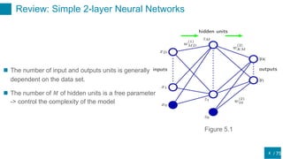
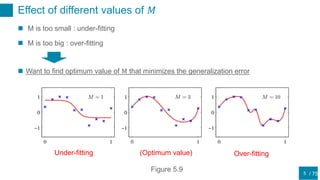
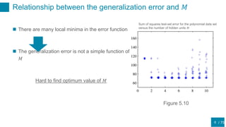
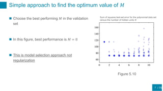
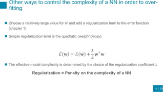
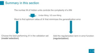
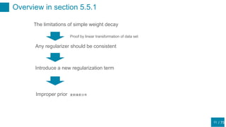
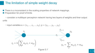
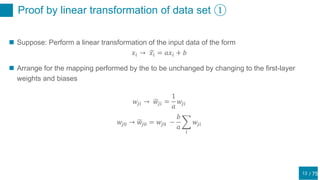
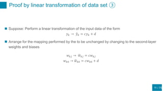
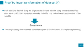
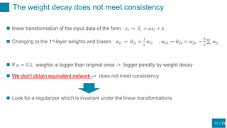
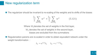
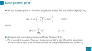
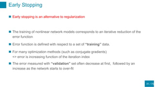
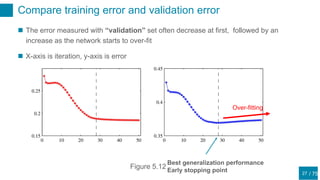
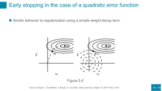
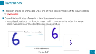
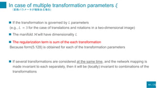
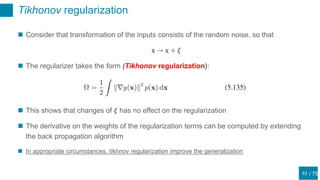
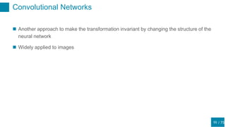
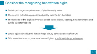
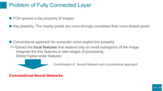
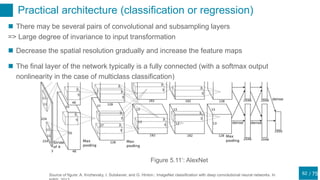
This document discusses regularization techniques for neural networks to prevent overfitting. It describes how the number of hidden units controls complexity and can lead to underfitting or overfitting. Early stopping is introduced as an alternative to regularization where training is stopped when validation error starts to increase. Consistency of regularization terms under linear transformations of data is discussed. Different approaches for building invariances like data augmentation, tangent propagation, and convolutional network structures are outlined.

1. / 75
PRML 5.5
Ryuta Shitomi
Optical Media Interface Lab
1

2. / 75
Table of Contents
• 5.5 Regularization in Neural Networks
• 5.5.1 Consistent Gaussian priors
• 5.5.2 Early Stopping
• 5.5.3 Invariances
• 5.5.4 Tangent propagation
• 5.5.5 Training with transformed data
• 5.5.6 Convolutional networks
• 5.5.7 Soft weight sharing
2

3. / 75
5.5 Regularization in Neural Networks
3

4. / 75
Review: Simple 2-layer Neural Networks
4
 The number of input and outputs units is generally
dependent on the data set.
 The number of 𝑀 of hidden units is a free parameter
-> control the complexity of the model
Figure 5.1

5. / 75
Effect of different values of 𝑀
5
 M is too small : under-fitting
 M is too big : over-fitting
 Want to find optimum value of M that minimizes the generalization error
(Optimum value)Under-fitting Over-fitting
Figure 5.9

6. / 75
Relationship between the generalization error and 𝑀
6
 There are many local minima in the error function
 The generalization error is not a simple function of
𝑀
Hard to find optimum value of 𝑀
Sum of squares test-set error for the polynomial data set
versus the number of hidden units 𝑀
Figure 5.10

7. / 75
Simple approach to find the optimum value of 𝑀
7
 Choose the best performing 𝑀 in the validation
set
 In this figure, best performance is 𝑀 = 8
 This is model selection approach not
regularization
Sum of squares test-set error for the polynomial data set
versus the number of hidden units 𝑀
Figure 5.10

8. / 75
Other ways to control the complexity of a NN in order to over-
fitting
8
 Choose a relatively large value for 𝑀 and add a regularization term to the error function
(chapter 1)
 Simple regularization term is the quadratic (weight decay)
𝐸 𝐰 = 𝐸 𝐰 +
λ
2
𝐰 𝑇
𝐰
 The effective model complexity is determined by the choice of the regularization coefficient λ
Regularization = Penalty on the complexity of a NN

9. / 75
Summary in this section
9
The number M of hidden units controls the complexity of a NN
Under-fitting VS over-fitting
Want to find optimum value of 𝑀 that minimizes the generalization error
Choose the best performing 𝑀 in the validation set
(model selection)
Add the regularization term in error function
(regularization)

10. / 75
5.5.1 Consistent Gaussian priors
10

11. / 75
Overview in section 5.5.1
11
The limitations of simple weight decay
Proof by linear transformation of data set
Any regularizer should be consistent
Introduce a new regularization term
Improper prior 変則事前分布

12. / 75
The limitation of simple weight decay
12
 There is a inconsistent in the scaling properties of network mappings.
 Preparation for proof of limits
・consider a multilayer perceptron network having two layers of weights and liner output
units
・input variables 𝐱 = 𝑥1, … , 𝑥𝑖, … , 𝑥 𝐷 , 𝐲 = 𝑦1, … , 𝑦 𝑘 … , 𝑦 𝐾
𝑧𝑗 = ℎ
𝑖
𝑤𝑗𝑖 𝑥𝑖 + 𝑤𝑗0
𝑧𝑗
𝑧𝑗
𝑧𝑗−1
𝑧𝑗+1
𝑦 𝑘
𝑦 𝑘 =
𝑗
𝑤 𝑘𝑗 𝑧𝑗 + 𝑤 𝑘0
Figure 5.1‘

13. / 75
Proof by linear transformation of data set ①
13
 Suppose: Perform a linear transformation of the input data of the form
𝑥𝑖 → 𝑥𝑖 = 𝑎𝑥𝑖 + 𝑏
 Arrange for the mapping performed by the to be unchanged by changing to the first-layer
weights and biases
𝑤𝑗𝑖 → 𝑤𝑗𝑖 =
1
𝑎
𝑤𝑗𝑖
𝑤𝑗0 → 𝑤𝑗0 = 𝑤𝑗0 −
𝑏
𝑎
𝑖
𝑤𝑗𝑖

14. / 75
Proof by linear transformation of data set ②
14
 Before linear transformation of the input data
𝑧𝑗 = ℎ
𝑖
𝑤𝑗𝑖 𝑥𝑖 + 𝑤𝑗0
𝑧𝑗 = ℎ 𝑤𝑗1 𝑥1 + 𝑤𝑗2 𝑥2 + … + 𝑤𝑗𝐷 𝑥 𝐷 + 𝑤𝑗0
 After linear transformation of the input data
𝑧𝑗 = ℎ 𝑤𝑗1 𝑎𝑥1 + 𝑏 + 𝑤𝑗2 𝑎𝑥2 + 𝑏 + … + 𝑤𝑗𝐷 𝑥 𝐷 + 𝑤𝑗0
𝑧𝑗 = ℎ 𝑤𝑗1 𝑎𝑥1 + 𝑤𝑗2 𝑎𝑥2 + … + 𝑤𝑗𝐷 𝑥 𝐷 + 𝑏 𝑤𝑗1 + 𝑤𝑗2 + … + 𝑤𝑗𝐷 + 𝑤𝑗0
𝑤𝑗𝑖 → 𝑤𝑗𝑖 =
1
𝑎
𝑤𝑗𝑖
𝑤𝑗0 → 𝑤𝑗0 = 𝑤𝑗0 −
𝑏
𝑎
𝑖
𝑤𝑗𝑖
Same output

15. / 75
Proof by linear transformation of data set ③
15
 Suppose: Perform a linear transformation of the input data of the form
𝑦 𝑘 → 𝑦 𝑘 = 𝑐𝑦 𝑘 + 𝑑
 Arrange for the mapping performed by the to be unchanged by changing to the second-layer
weights and biases
𝑤 𝑘𝑗 → 𝑤 𝑘𝑗 = 𝑐𝑤 𝑘𝑗
𝑤 𝑘0 → 𝑤 𝑘0 = 𝑐𝑤 𝑘0 + 𝑑

16. / 75
Proof by linear transformation of data set ④
16
 If we train one network using the original data and one network using linearly transformed
data, we should obtain equivalent networks that differ only by the linear transformation of the
weights
Consistency
 The weight decay does not meet consistency ( one of the limitations of simple weight decay)

17. / 75
The weight decay does not meet consistency
17
 linear transformation of the input data of the form : 𝑥𝑖 → 𝑥𝑖 = 𝑎𝑥𝑖 + 𝑏
 Changing to the 1st-layer weights and biases : 𝑤𝑗𝑖 → 𝑤𝑗𝑖 =
1
𝑎
𝑤𝑗𝑖 , 𝑤𝑗0 → 𝑤𝑗0 = 𝑤𝑗0 −
𝑏
𝑎 𝑖 𝑤𝑗𝑖
 If 𝑎 = 0.1, weights is bigger than original ones -> bigger penalty by weight decay
 We don’t obtain equivalent network -> does not meet consistency
 Look for a regularizer which is invariant under the linear transformations

18. / 75
New regularization term
18
 The regularizer should be invariant to re-scaling of the weights and to shifts of the biases
λ1
2
𝑤∈𝒲1
𝑤2
+
λ2
2
𝑤∈𝒲2
𝑤2
(5.121)
Where 𝒲1denotes the set of weights in the first layer,
𝒲2 denotes the set of weights in the second layer,
biases are excluded from the summations
 Regularization params are re-scaled in order to obtain equivalent network under the
weight transformation :
λ1 → 𝑎1/2
𝜆1 λ2 → 𝑐−1/2
λ2

19. / 75
Improper prior (変則事前分布)
19
 The regularizer (5.121) corresponds to a prior of the form (improper prior):
𝑝 𝐰 𝛼1, 𝛼2 ∝ exp −
𝛼1
2
𝑤∈𝒲1
𝑤2
−
𝛼2
2
𝑤∈𝒲2
𝑤2
(5.122)
 Priors of this form are improper because the bias params are unconstrained
 Disadvantage:
=> difficulties in selecting regularization coefficients
=> difficulties in model comparison within Bayesian framework ( the correspondingevidence is
zero) (for more detail, see 5.7)
 (Therefore) include separate priors for the biases having their own hyperparameters

20. / 75
More general prior
20
 We can consider priors in which the weights are divided into any number of groups 𝒲𝑘 :
𝑝 𝐰 ∝ exp −
1
2
𝑘
𝛼 𝑘 𝐰 𝑘
2
5.123
where
𝐰 𝑘
2
=
𝑗∈𝒲 𝑘
𝑤𝑗
2
(5.124)
 Automatic relevance determination (ARD see Section 7.2.2 )
We choose the groups in this priors to correspond to the sets of weights associated
with each of the input units, and we optimize the marginal likelihood with params αk

21. / 75
𝑥
𝑧𝑖
𝑦
𝑤𝑖1
𝑤𝑖0 𝑤10
𝑤1𝑗
Example of general prior in two-layer NN
21
 Single input 𝑥, 12hidden layer having ‘tanh’ activation function and single output 𝑦 in two-
layer NN
𝑧𝑖 = tanh 𝑤𝑖1 𝑥 + 𝑤𝑖0 𝑖 = 1, … , 12
𝑦 =
𝑗=1
12
𝑤1𝑗 𝑧𝑗 + 𝑤10
𝑧 = tanh(𝑤x)
Figure 5.2’ Figure 5.3’

22. / 75
Example of general prior in two-layer NN
22
 Define the priors
𝑝 𝑤𝑖1 ∝ exp −
1
2
𝛼1
w
𝑤𝑖1
2
(1st layer weights)
𝑝 𝑤𝑖0 ∝ exp −
1
2
𝛼1
b
𝑤𝑖0
2
(1st layer biases)
𝑝 𝑤1𝑗 ∝ exp −
1
2
𝛼2
w
𝑤1𝑗
2
(2nd layer weights)
𝑝 𝑤1𝑗 ∝ exp −
1
2
𝛼2
w
𝑤1𝑗
2
(2nd layer bias)
 𝛼1
w
, 𝛼1
b
, 𝛼2
w
, 𝛼2
b
is hyperparameters, which represent
the precisions of the Gaussian distribution (if 𝛼 is
bigger, tail is spread)
Figure 1.13

23. / 75
Figure . Example of general prior in two-layer NN
23Figure 5.11

24. / 75
5.5.2 Early Stopping
24

25. / 75
Early Stopping
25
 Early stopping is an alternative to regularization
 The training of nonlinear network models corresponds to an iterative reduction of the
error function
 Error function is defined with respect to a set of “training” data.
 For many optimization methods (such as conjugate gradients)
=> error is increasing function of the iteration index
 The error measured with “validation” set often decrease at first, followed by an
increase as the network starts to over-fit

26. / 75
Compare training error and validation error
26
 The error measured with “validation” set often decrease at first, followed by an
increase as the network starts to over-fit
 X-axis is iteration, y-axis is error
Over-fitting
Best generalization performance
Early stopping point
Figure 5.12

27. / 75
Compare training error and validation error
27
 The error measured with “validation” set often decrease at first, followed by an
increase as the network starts to over-fit
 X-axis is iteration, y-axis is error
Over-fitting
Best generalization performance
Early stopping point
Figure 5.12

28. / 75
Early stopping in the case of a quadratic error function
28
 Similar behavior to regularization using a simple weight-decay term
Source of figure: I. Goodfellow, Y. Bengio, A. Courville,: Deep Learning chapter 7.8, MIT Press, 2016
Figure 5.4’

29. / 75
5.5.3 Invariances
29

30. / 75
Invariances
30
 Prediction should be unchanged under one or more transformations of the input variables
=> invariances
 Example) classification of objects in two-dimensional images
・translation invariance : unchanged under position transformation within the image
・scale invariance: unchanged under scale transformation
Position transformation
Scale transformation
Figure 5.5’

31. / 75
Invariances in case that sufficiently large training set is
available
31
 Adaptive model such as a NN can learn the invariance, at least approximately
 It requires that various transformations are included in the training data
 To realize translation invariance in an image, the training set should include examples of
objects at many different positions
 This approach may be impractical if training examples is limited, or if there are several
invariants( the number of combinations of transformations grows exponentially )

32. / 75
4 alternative approaches for making adaptive model have
invariances
32
 1. Data augmentation (データ拡張)
 2. Add the regularization term in error function that penalizes changes in the model output
when the input is transformed => tangent propagation
 3. Invariance is built in pre-processing by extracting features that are invariant under the
required transformations
 4. Build the invariance properties into the structure of a NN
=> to realize this, the use of local receptive fields and shared weights(discussed in 5.5.6, 7)

33. / 75
Approach1. Data augmentation
33
 Augment the training data according to the desired invariance => improve generalization
 Advantages
・Relatively easy to implement
・For sequential training methods, we can transform the input pattern before feeding the
model => when the same pattern are used, a different transformation is added
・For batch methods, obtain similar effect by replicating each data points a number of
times and transforming each copy independently
 Disadvantages => computational cost increase
Original data Data augmentation
NNs
Neural Networks
Figure 5.6’

34. / 75
Approach1. Data augmentation
34
 Augmentation can be used to encourage complex invariances
Original image
Displacement fields are generated by sampling random displacements
And smoothing by convolution with Gaussians of width 0.01, 30 and 60
Figure 5.14

35. / 75
Approach 3. Pre-processing for invariances (前処理)
35
 Invariance is built in pre-processing by extracting features that are invariant under the required
transformations
 Advantage
・Using such pre-processed features as input, any regression or classification system will also
respect these invariances.
 Disadvantage
・it can be difficult to find hand-crafted useful features with the required invariances

36. / 75
5.5.4 Tangent Propagation
36

37. / 75
Tangent Propagation
37
 Motivation: We don’t want to change the output when the input changes
 Add the regularization term in error function that penalizes changes in the model output when
the input is transformed
 Derivation of tangent propagation
Consider the effect of a transformation on a particular input vector 𝐱 𝑛
If transformation is continuous (e.g. translation or rotation, not mirror reflection), the transformed
patterns exist on the manifold ℳ within the 𝐷-dimensional input space

38. / 75
Derivation of tangent propagation ①
38
 Consider the case of 𝐷 = 2
 The transformation is governed by a single parameter 𝜉
 The subspace ℳ composed by 𝐱 𝑛 is one-dimensional, and parameterized by 𝜉
 Each point on the manifold ℳ can be represented by a vector 𝐬 𝐱 𝑛, 𝜉
=> 𝐬 𝐱 𝑛, 0 ≜ 𝐱 𝑛
𝜉 = 0
Figure 5.15

39. / 75
Derivation of tangent propagation ②
39
 The tangent to the curve ℳ is given by the direction derivative 𝛕 = 𝜕𝐬/𝜕𝜉
 The tangent vector at point 𝐱 𝑛 is given by:
 Transforming the input also changes the output
(入力を変化させると出力も変化する)
 The derivative of output unit 𝑘 with respect to 𝜉 is given by:
Figure 5.15

40. / 75
Derivation of tangent propagation ③
40
 Transforming the input also changes the output
 The derivative of output unit 𝑘 with respect to 𝜉 is given by:
𝜉
outputinput
𝑦 𝑘
𝜕𝑦 𝑘
𝜕𝐱
𝜕𝑥𝑖
𝜕𝜉
 𝐽 𝑘𝑗 is the element of the Jacobian matrix 𝐉 (discussed in section 5.3.4)
Figure 5.6’

41. / 75
Derivation of tangent propagation ④
41
 Add the result (5.126) to the standard error function 𝐸
 This encourage local invariance in the neighborhood of the data points
 Modified error function 𝐸 is given by:
𝐸 = 𝐸 + λΩ
where λ is a regularization coefficient and the regularization function Ω :
 The regularization function will be zero when model have invariance under the
transformation in the neighborhood of each pattern vector.
 λ controls the balance between fitting the training data and learning the invariance
property

42. / 75
How to implement actually
42
 We have to calculate the regularization function Ω
 Calculate Jacobian 𝐉 using backpropagation
 Calculate approximately tangent vector 𝛕 using finite differences
This form is used actually

43. / 75
Calculate tangent vector 𝛕 using finite differences
43
 Transformation using a small value 𝜉′
 Subtracting the original vector 𝐱 𝑛 from the transformed vector 𝐬(𝐱 𝑛, 𝜉′
)
𝛕 𝑛 =
𝐬 𝐱 𝑛, 𝜉′
− 𝐬 𝐱 𝑛, 0
𝜉′
=
𝐬 𝐱 𝑛, 𝜉′
− 𝐱 𝑛
𝜉′
Original 𝐱 𝑛
Infinitesimal clockwise rotation
𝛕 𝑛
𝐱 𝑛 + 15𝛕 𝑛
Can regard that image
rotated 15 degrees
True rotated
image
Figure 5.15
Figure 5.16

44. / 75
In case of multiple transformation parameters 𝜉
（変換パラメータが複数ある場合)
44
 If the transformation is governed by 𝐿 parameters
(e.g., 𝐿 = 3 for the case of translations and rotations in a two-dimensional image)
 The manifold ℳwill have dimensionality 𝐿
 The regularization term is sum of the each transformation
Because form(5.128) is obtained for each of the transformation parameters
 If several transformations are considered at the same time, and the network mapping is
made invariant to each separately, then it will be (locally) invariant to combinations of the
transformations

45. / 75
5.5.5 Training with transformed data
45

46. / 75
Training with transformed data
46
(Review): One approach to encourage invariance of a model to a set of transformations is
data augmentation
 Data augmentation is closely related to the technique of tangent propagation

47. / 75
Formulation of data augmentation ①
47
 As in section 5.5.4, we define the function 𝐬 𝐱, 𝜉 , with 𝐬 𝐱, 0 ≜ 𝐱
 We consider a sum-of-squares error function for single output, and the error function for
untransformed inputs is written by (in the infinite data set limit):
 Consider an infinite number of copies of data points, each of which is transformed by 𝜉,
and 𝜉 is generated from distribution 𝑝(𝜉)
 Assume 𝑝(𝜉) is to be mean zero and the variance is small.
 The error function for this expanded data set is written by:

48. / 75
Formulation of data augmentation ②
48
 Expand the transformation function 𝐬 𝐱, 𝜉 as a Taylor series in power of 𝜉 to give:
where 𝛕′ denotes the second derivative of 𝐬(𝐱, 𝜉) with respect to 𝜉 evaluated at 𝜉 = 0
 Using this, model function 𝑦(𝐬(𝐱, 𝜉) is given by:

49. / 75
Formulation of data augmentation ③
49
 When we substitute model function into the mean error function (5.130) :
Additional
Terms by
transformation
𝔼 𝜉 = 0

50. / 75
Formulation of data augmentation ④
50
 If we denote 𝔼 𝜉2
by λ and omit terms of 𝑂(𝜉3
), error function 𝐸 is written by:
where 𝐸 is original sum-of-squares error function, and the regularization term Ω (Integrate
with respect to 𝑡 is:

51. / 75
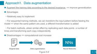
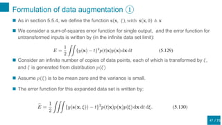
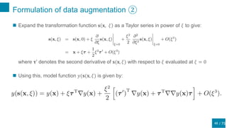
Formulation of data augmentation ⑤
51
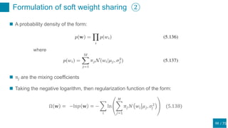
 The function that minimizes the sum-of-squares error is the conditional mean 𝐸[𝑡|𝐱]
 (5.131) is the original sum-of-squares-error plus terms of 𝑂(𝜉2
)
 Therefore， the model function that minimizes the (5.131) will have the form:
 For 𝑂 𝜉2
, the first term of the regularization term Ω is zero
 Thus, regularization term Ω can be written by:

52. / 75
Compare the tangent propagation regularizer
52
 Tangent propagation regularizer:
 Formulation of data augmentation:

53. / 75
Tikhonov regularization
53
 Consider that transformation of the inputs consists of the random noise, so that
𝐱 → 𝐱 + 𝝃
 The regularizer takes the form (Tikhonov regularization):
 This shows that changes of 𝝃 has no effect on the regularization
 The derivative on the weights of the regularization terms can be computed by extending
the back propagation algorithm
 In appropriate circumstances, tikhnov regularization improve the generalization

54. / 75
5.5.6 Convolutional networks
54

55. / 75
Convolutional Networks
55
 Another approach to make the transformation invariant by changing the structure of the
neural network
 Widely applied to images

56. / 75
Consider the recognizing handwritten digits
56
 Each input image comprises a set of pixel intensity value
 The desired output is a posterior probability over the ten digit class
 The identity of the digit is invariant under translations , scaling, small rotations and
subtle transformations
 Simple approach: input the flatten image to fully connected network (FCN)
 FCN would learn appropriate invariances if given a sufficiently large training set

57. / 75
Problem of Fully Connected Layer
57
 FCN ignores a key property of images
 Key property: The nearby pixels are more strongly correlated than more distant pixels
 Conventional approach for computer vision exploit this property
=> Extract the local features that depend only on small subregions of the image
Integrate the this features in later stages of processing
Detect higher-order features
Combination of Neural Network and conventional approach
Convolutional Neural Networks

58. / 75
3 notions into convolutional neural networks
58
 1. Local receptive field
 2. weight sharing
 3. subsampling
 CNN consists the 2 layers
1. Convolutional layer
・local receptive field
・weight sharing
2. Subsampling layer
・subsampling
・local receptive field
Figure 5.17

59. / 75
Convolutional layer
59
 Units in a feature map are constrained to share the same
weight value
 If each unit take inputs from a 3x3 pixel patch of the
image, feature map has 9 adjustable weight params and
one adjustable param
 One feature map detects same pattern at different
locations in the input image
 Convolution of the image pixel intensities with a ‘kernel’
comprising the weight params
Source of figure 5-1’: https://github.com/vdumoulin/conv_arithmetic
Feature map
Figure 5.7’
3x3 Weight

60. / 75
Subsampling layer
60
 The inputs to the subsampling layer is the output
of the convolutional units
 Recently, the famous subsampling layer are
・max-pooling layer
・average-pooling layer
 If receptive field is 2x2 and nonoverlapping,
there are half the number of rows and columns Figure 5.8’: example of subsampling
Source of figure 5- : https://cs231n.github.io/convolutional-networks/
Unit
Receptive field

61. / 75
Invariances
61
 Convolutional layer
translations and distortions of the inputs
Source of figure 5- : https://cs231n.github.io/convolutional-networks/
 Subsampling layer
translations and scaling
Figure 5.9’
It just shifts the active units
Figure 5.10’

62. / 75
Practical architecture (classification or regression)
62
 There may be several pairs of convolutional and subsampling layers
=> Large degree of invariance to input transformation
 Decrease the spatial resolution gradually and increase the feature maps
 The final layer of the network typically is a fully connected (with a softmax output
nonlinearity in the case of multiclass classification)
Figure 5.11’: AlexNet
Source of figure: A. Krizhevsky, I. Sutskever, and G. Hinton.: ImageNet classification with deep convolutional neural networks. In

63. / 75
Train of convolutional neural networks
63
 Using the slightly modified backpropagation algorithm to satisfy the constraints
 The number of weights in the network is smaller than if the network were fully connected
 Due to the constraints (weight sharing), the number of independent trainable parameters
is much smaller

64. / 75
5.5.7 Soft weight sharing
64

65. / 75
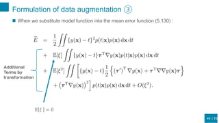
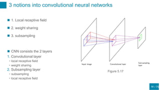
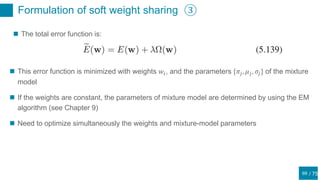
Problem of weight sharing
65
 Weight sharing technique (Section 5.5.6)
=>Add the constraint that weights belonging to the same
groups are equal
 “This approach is effective when the problem being
addressed is quite well understood, so that it is possible
to specify, in advance, which weights should be
identical.”[1]
e.g.) Consider the recognizing handwritten digits, wealready
know the some invariances
[1]. Nowlan, S.J. and G.E. Hinton,: Simplifying neural networks by soft weight sharing. Neural Computation 4(4), 473-
Figure 5.17
We know that we should share the weights each ker
Soft weight sharing
If we don’t know the where we should share the weights

66. / 75
Overview of soft weight sharing
66
 Add the regularization term
 Regularization term encourages weights belonging to the same groups to have similar
values
 Learnable:
・weights
・grouping of the weights
・mean weight value for each group
・spread of values within the groups
Figure 2.22
Group1
Group2
Group3

67. / 75
Formulation of soft weight sharing ①
67
 Recall: the simple weight decay regularizer can be viewed as the negative log of a
Gaussian prior distribution over the weights
 Consider the each weight belongs to several groups
=> probability over the weight define as a mixture of Gaussians
 Mean and variances of the Gaussian components and the mixing coefficients are
determined as part of the learning process

68. / 75
Formulation of soft weight sharing ②
68
 A probability density of the form:
where
 π𝑗 are the mixing coefficients
 Taking the negative logarithm, then regularization function of the form:
Ω 𝐰 = −ln𝑝 𝐰 = −
𝑖
ln
𝑗=1
𝑀
𝜋𝑗 𝒩 𝑤𝑖 𝜇 𝑗, 𝜎𝑗
2
(5.138)

69. / 75
Formulation of soft weight sharing ③
69
 The total error function is:
 This error function is minimized with weights 𝑤𝑖, and the parameters {𝜋𝑗, 𝜇 𝑗, 𝜎𝑗} of the mixture
model
 If the weights are constant, the parameters of mixture model are determined by using the EM
algorithm (see Chapter 9)
 Need to optimize simultaneously the weights and mixture-model parameters

70. / 75
Derivatives with respect to the weights ①
70
 The mixture coefficient {𝜋𝑗} is considered as prior probability for group 𝑗
 The posterior probabilities over the mixture coefficient :
𝛾𝑗 𝑤𝑖 = 𝑝 𝑔𝑟𝑜𝑢𝑝 = 𝑗 𝑤𝑖) =
𝑝 𝑔𝑟𝑜𝑢𝑝 = 𝑗 𝑝 𝑤𝑖 𝑔𝑟𝑜𝑢𝑝 = 𝑗
𝑝(𝑤𝑖)

71. / 75
Derivatives with respect to weights ②
71
 The derivatives of the total error function with respect to weights is:
𝜕
𝜕𝑤𝑖
log 𝑝 𝑤𝑖 =
1
𝑝 𝑤𝑖
𝜕
𝜕𝑤𝑖
𝑝 𝑤𝑖 =
1
𝑝 𝑤𝑖
𝑗
𝜋𝑗
𝜕
𝜕𝑤𝑖
𝒩 𝑤𝑖 𝜇 𝑗, 𝜎2
𝜕
𝜕𝑥
𝒩 𝑥 𝜇, 𝜎2
= 𝒩 𝑥 𝜇, 𝜎2
−
𝑥 − 𝜇
𝜎2
References
 The regularization term encourages each weight to pull towards the centre of the 𝑗th
gaussian

72. / 75
Derivatives with respect to the centres of the Gaussians
72
 Derivatives of the error function with respect to the centres of the Gaussians is:
 Push 𝜇 𝑗 towards an average of the weight values
References
𝜕
𝜕𝜇
𝒩 𝑥 𝜇, 𝜎2
= 𝒩 𝑥 𝜇, 𝜎2
𝑥 − 𝜇
𝜎2
𝜕
𝜕𝜇 𝑗
ln𝑝 𝑤𝑗 =
𝑖
𝜕
𝜕𝜇 𝑗
ln 𝑝 𝑤𝑖

73. / 75
Derivatives with respect to the variances of the Gaussians
73
 Derivatives of the error function with respect to the variances of the Gaussians is:
 Drive 𝜎𝑗 towards the weighted average of the squared deviations of the weights
around corresponding centre 𝜇 𝑗
References
𝜕
𝜕𝜎
𝒩 𝑥 𝜇, 𝜎2 = 𝒩 𝑥 𝜇, 𝜎2 −
1
𝜎
+
𝑥 − 𝜇 2
𝜎3
𝜕
𝜕𝜎𝑗
ln𝑝 𝑤𝑖 =
𝑖
𝜕
𝜕𝜎𝑗
ln 𝑝 𝑤𝑖

74. / 75
Practical implementation of the variances
74
 The variances 𝜎2
must be positive
 New variables 𝜂 𝑗 defined by:
 Prevent some variances 𝜎2
going to zero (see Section 9.2.1)

75. / 75
Practical implementation of the mixing coefficients 𝜋𝑗
75
 Need to take account of the below constraints :
 Define a set of auxiliary variables {𝜂 𝑗} using the 𝑠𝑜𝑓𝑡𝑚𝑎𝑥 function given by :
 The derivatives of the regularized error function with respect to the {𝜂 𝑗}
 𝜋𝑗 is driven towards the average posterior probability for component 𝑗