Review research on semi-supervised learning, self-supervised learning and contrastive learnings

1. https://clarken92.github.io/
https://scholar.google.com.au/citations?user=aD6y8joAAAAJ&hl=en
https://www.linkedin.com/in/kien-do-b45846a4
Towards Label and Data Efficient
Deep Learning
Dr. Kien Do
A2I2, Deakin University, Australia

2. 3/16/2022 2
https://innovativeadagency.com/blog/importance-data-collection/
Data are abundant online and can be obtained freely

3. 3/16/2022 3
However, annotating them is often expensive and time consuming
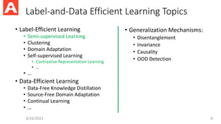
=> We should think more about label efficient learning
https://appen.com/blog/data-annotation/
https://medicalxpress.com/news/2017-10-dementia-costly.html
https://www.roastycoffee.com/coffee-makes-me-tired/

4. Yann LeCun’s Cake
3/16/2022 4
https://syncedreview.com/2019/02/22/yann-lecun-cake-analogy-2-0/

5. 3/16/2022 5
m.facebook.com/mldcmu/photos/quoting-professor-lecun-april-30-2019-i-now-call-it-self-supervised-learning-bec/2178914695721030/
But unsupervised learning is what most humans and animals do

6. Label-and-Data Efficient Learning Topics
• Label-Efficient Learning
• Semi-supervised Learning
• Clustering
• Domain Adaptation
• Self-supervised Learning
• Contrastive Representation Learning
• …
• …
• Data-Efficient Learning
• Data-Free Knowledge Distillation
• Source-Free Domain Adaptation
• Continual Learning
• …
3/16/2022 6
• Generalization Mechanisms:
• Disentanglement
• Invariance
• Causality
• OOD Detection

7. Semi-supervised Learning
3/16/2022 7

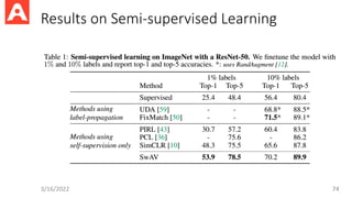
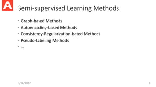
8. Semi-supervised Learning (SSL)
• Problem: Combine labeled and unlabeled data (usually >= 90% of the
data) to train a model
• Assumptions:
• Smoothness Assumption
• Cluster Assumption
• Manifold Assumption
3/16/2022 8
Semi-Supervised Learning, Chapelle et al., 2006

9. Semi-supervised Learning Methods
• Graph-based Methods
• Autoencoding-based Methods
• Consistency-Regularization-based Methods
• Pseudo-Labeling Methods
• …
3/16/2022 9

10. Label Propagation (Zhu and Ghahramani, 2004)
• Assume nonnegative similarity scores between samples
• Construct an undirected graph over all nodes with edges weighted by
similarity scores.
• Perform the following steps until convergence:
• Propagate labels: , where is the transition matrix
• Set the class probability of labeled data to the ground-truth
3/16/2022 10

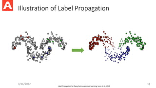
11. Illustration of Label Propagation
3/16/2022 11
Label Propagation for Deep Semi-supervised Learning, Iscen et al., 2019

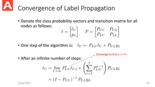
12. Convergence of Label Propagation
• Denote the class probability vectors and transition matrix for all
nodes as follows:
• One step of the algorithm is:
• After an infinite number of steps:
3/16/2022 12
Converge to 0 as t -> ∞

13. Label Propagation as Energy Minimization
• The energy function:
where is the graph Laplacian.
3/16/2022 13
smoothness
regularization
label constraint
solution is a harmonic
function satisfying the
Laplace’s equation:

14. Problems of Label Propagation (LP)
• LP is transductive, thus, cannot handle new samples.
• LP requires matrix inversion for the exact solution, which is usually
costly in practice.
3/16/2022 14

15. Label Propagation + Gaussian Mixture Model
• Intuition: GMM provides the local fit to data while LP ensures the
global manifold structure.
3/16/2022 15
Implicitly assume that
#mixtures ≠ #classes
GMM

16. ELBO of GMM
3/16/2022 16

17. GMM Training and Label Inference
• We can train the GMM via the EM algorithm
• After EM converges, we can predict the label as:
3/16/2022 17

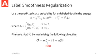
18. Label Smoothness Regularization
Use the predicted class probability for unlabeled data in the energy
where
Finetune by maximizing the following objective:
3/16/2022 18
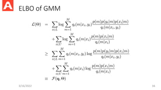
ELBO

19. Training Procedure for LP+GMM
• Train all parameters of p(m), p(x|m), p(y|m) by maximizing via the
standard EM algorithm.
• Fix p(m), p(x|m) and train p(y|m) by maximizing .
3/16/2022 19

20. Some illustrative results
3/16/2022 20

21. Problems of LP + GMM
• EM algorithm is not applicable to high dimensional data like images.
• This method still requires full batch updates.
3/16/2022 21

22. Semi-VAE (Kingma et al., 2014)
3/16/2022 22
Generative Model Inference Model

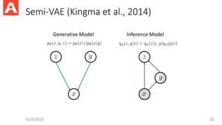
23. Training Objective for Semi-VAE
• ELBO on labeled data:
• ELBO on unlabeled data:
• Final objective:
3/16/2022 23
Weight the NLL by soft-label Avoid over-confident predictions
Both y and z are used to predict x

24. Results
3/16/2022 24
Can some how separate style from class
Not very good

25. Problems of Semi-VAE
• It is a generative model while the classification problem is
discriminative.
• => It may be better to perform SSL with discriminative model only
• It has no mechanism to ensure that the decoder must use both y and
z to reconstruct x. If z is a big vector, the decoder may just use z.
• => A possible solution is making y and z independent: I(y, z) = 0
3/16/2022 25
Disentanglement

26. Pi-model
3/16/2022 26
Input augmentation function
Classifier
Ramp-up function
Number of classes

27. Temporal Ensembling
3/16/2022 27
Store z of each sample in a memory and update it with momentum:
Update is delayed
until the next epoch

28. Mean Teacher (MT)
3/16/2022 28
Teacher plays the
role of an ensemble
Cross-entropy loss

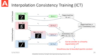
29. Interpolation Consistency Training (ICT)
3/16/2022 29
Can be consider as a lineartiy
regularization of f
Smoothness due to bounded Lipschitz constant
Interpolation Consistency Training for Semi-Supervised Learning, Verma et al., 2019

30. Training Procedure of ICT
3/16/2022 30
Mixup as
consistency loss
Like mean teacher
These samples from the teacher model
Train student model

31. Intuitions
• Intuitions:
• Learn a smooth input-output manifold by forcing the classifier to give
consistent predictions for inputs under simple perturbations.
• Can we have better data and weight perturbations?
3/16/2022 31

32. Maximum Uncertainty Regularization (MUR)
• Under weak data perturbation, is often close to .
The classifier can only learn a locally smooth mapping from to .
• We want to be: i) not too close to , and ii) difficult for the
classifier to predict correctly.
• We choose to be a maximum uncertain (w.r.t. ) virtual point:
32
3/16/2022 Semi-Supervised Learning with Variational Bayesian Inference and Maximum Uncertainty Regularization, Do et al., 2020

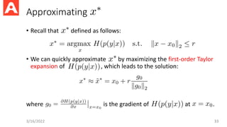
33. Approximating
• Recall that defined as follows:
• We can quickly approximate by maximizing the first-order Taylor
expansion of , which leads to the solution:
where is the gradient of at .
33
3/16/2022

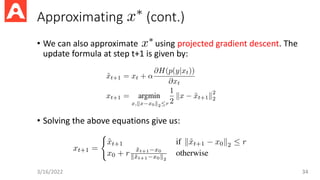
34. Approximating (cont.)
• We can also approximate using projected gradient descent. The
update formula at step t+1 is given by:
• Solving the above equations give us:
34
3/16/2022

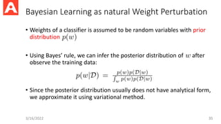
35. Bayesian Learning as natural Weight Perturbation
• Weights of a classifier is assumed to be random variables with prior
distribution
• Using Bayes’ rule, we can infer the posterior distribution of after
observe the training data:
• Since the posterior distribution usually does not have analytical form,
we approximate it using variational method.
3/16/2022 35

36. Variational Bayesian Inference (VBI)
3/16/2022 36
Control the model’s complexity
Control the data misfit
Like ensemble methods
Use Variational Dropout to
facilitate this sampling
Note: p(w) is chosen to be the log-uniform distribution by Kingma et al., 2014 and it was shown to be pathological by many
works. However, it cannot be easily replaced [1] and still work well in practice. For a better alternative, please check [2].
[1]: Variational Bayesian dropout: pitfalls and fixes, Hron et al., 2018
[2]: Structured Dropout Variational Inference for Bayesian Neural Networks, Nguyen et al., 2021

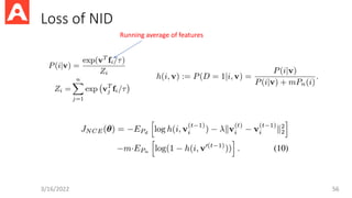
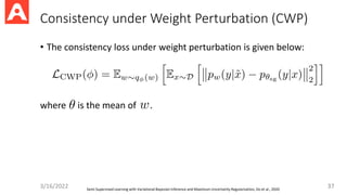
37. Consistency under Weight Perturbation (CWP)
• The consistency loss under weight perturbation is given below:
where is the mean of .
37
3/16/2022 Semi-Supervised Learning with Variational Bayesian Inference and Maximum Uncertainty Regularization, Do et al., 2020

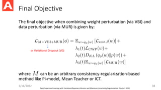
38. Final Objective
The final objective when combining weight perturbation (via VBI) and
data perturbation (via MUR) is given by:
where can be an arbitrary consistency-regularization-based
method like Pi-model, Mean Teacher or ICT.
38
3/16/2022
Semi-Supervised Learning with Variational Bayesian Inference and Maximum Uncertainty Regularization, Do et al., 2020
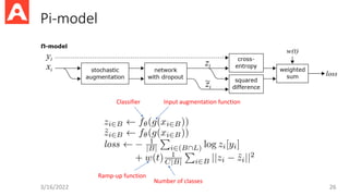
or Variational Dropout (VD)

39. Results on CIFAR-10/100 and SVHN
39
SVHN

40. Ablation Study
40
Different coefficient values of ( )

41. Ablation Study (cont.)
41
Performance with different radiuses Random perturbation vs. MUR
The best value
of radius

42. Visualization of most uncertain samples
42

43. MixMatch
3/16/2022 43
Then they perform Mixup between labeled and unlabeled

44. Importance of Data Augmentation in SSL
• Consistency-Regularization-based methods like Pi-model, Mean
Teacher, ICT, MixMatch use only simple (weak) data augmentation.
• MUR can provide some help but still cannot replace good data
augmentation.
3/16/2022 44

45. UDA
3/16/2022 45
Strong data augmentation

46. Results of UDA
3/16/2022 46

47. FixMatch
3/16/2022 47

48. Objective Function of FixMatch
3/16/2022 48
weak augmentation
strong augmentation
unlabeled/labeled ratio threshold

49. Results of FixMatch
3/16/2022 49
Very close to supervised learning

50. Ablation Study of FixMatch
3/16/2022 50

51. Contrastive Learning
3/16/2022 51

52. Contrastive Learning in old days
• Triplet loss
• Max-margin distance metric:
3/16/2022 52

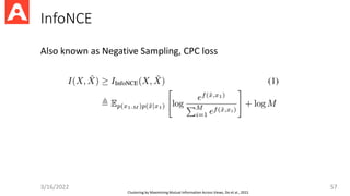
53. NCE
• We want to estimate/model the distribution
• Assume we have a noise distribution as reference
=> Transforming into binary classification
3/16/2022 53
P(C=0)/P(C=1)
Noise Constrastive Estimation, Ke Tran

54. NCE Loss
3/16/2022 54

55. Non-parametric Instance Discriminator (NID)
3/16/2022 55

56. Loss of NID
3/16/2022 56
Running average of features

57. InfoNCE
3/16/2022 57
Clustering by Maximizing Mutual Information Across Views, Do et al., 2021
Also known as Negative Sampling, CPC loss

58. SimCLR
3/16/2022 58

59. Results with different data augmentations
3/16/2022 59
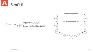
SimCLR significantly
depends on data
augmentation

60. Results with different batch size
3/16/2022 60
SimCLR significantly
depends on batch size

61. Advantages and Drawbacks of SimCLR
• Advantages:
• Simple to implement and use
• Drawbacks:
• Requires large batch size
• Memory intensive <= Addressed by MoCo
3/16/2022 61

62. MoCo
3/16/2022 62
When run on standard 8 GPU
machines, SimCLR can only
handle 1024 negative samples

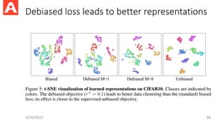
63. Debiased Contrastive Learning
• Sampling bias of standard contrastive loss: Negative samples can be
drawn from the same class as positive samples
3/16/2022 63
Negative distribution Weighting parameter

64. 3/16/2022 64
A practical debiased form based on the
asymptotic form of unbiased loss when N -> ∞
Debiased Contrastive Loss

65. Results
3/16/2022 65

66. Debiased loss leads to better representations
3/16/2022 66

67. BYOL
3/16/2022 67
Bootstrap your own latent: A new approach to self-supervised learning, Grill et al., 2020
An autoencoder
Stop gradient

68. Results with different batch sizes and data
augmentations
3/16/2022 68

69. Advantages and Drawbacks of BYOL
• Advantages:
• Eliminate the need for negative samples in standard contrastive loss
• Less depends on batch size and data augmentation compared to SimCLR
• Drawbacks:
• Learned representations can be collapsed to the same vector if:
• No prediction network is used
• No gradient stop is enforced on the target (EMA) branch
3/16/2022 69

70. SwAV
3/16/2022 70
normalized feature
code
prototype

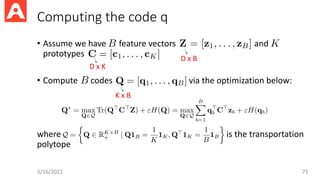
71. Computing the code q
• Assume we have feature vectors and
prototypes
• Compute codes via the optimization below:
where is the transportation
polytope
3/16/2022 71
D x B
D x K
K x B

72. Computing the code q (cont.)
• The optimal soft codes Q takes the form of a normalized exponential
matrix:
where and are renormalization vectors in and , respectively.
and are computed using the iterative Sinkhorn-Knopp algorithm.
3/16/2022 72

73. Linear classification results
3/16/2022 73

74. Results on Semi-supervised Learning
3/16/2022 74

75. Results with small batch sizes
3/16/2022 75

76. Advantages and Drawbacks of SwAV
• Advantages:
• Does not require negative samples, thus run faster than other methods
• Drawbacks:
• Requires some tricks to avoid collapse such as class balancing, which can
sometimes be violated in real situation
3/16/2022 76

77. Applications of Contrastive
Learning
3/16/2022 77

78. Self-Match
3/16/2022 78
SimCLR, MoCo, …
FixMatch

79. Results of Self-Match
3/16/2022 79
No results on
ImageNet

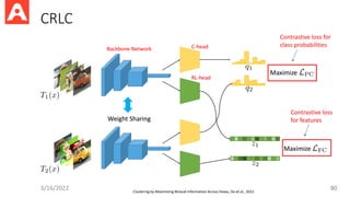
80. CRLC
3/16/2022 80
Contrastive loss for
class probabilities
Contrastive loss
for features
Clustering by Maximizing Mutual Information Across Views, Do et al., 2021

81. Training Objective of CRLC
3/16/2022 81
People usually choose f
to be a cosine similarity
but is it a good critic?

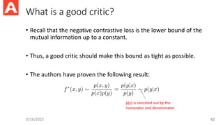
82. What is a good critic?
• Recall that the negative contrastive loss is the lower bound of the
mutual information up to a constant.
• Thus, a good critic should make this bound as tight as possible.
• The authors have proven the following result:
3/16/2022 82
p(y) is canceled out by the
numerator and denominator

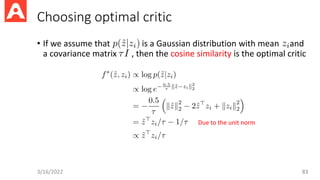
83. Choosing optimal critic
• If we assume that is a Gaussian distribution with mean and
a covariance matrix , then the cosine similarity is the optimal critic
3/16/2022 83
Due to the unit norm

84. Choosing optimal critic (cont.)
• The optimal critic is the log-of-dot-product function:
3/16/2022 84
May not be theoretically
equivalent is a practically
good approximation

85. Clustering Results
3/16/2022 85

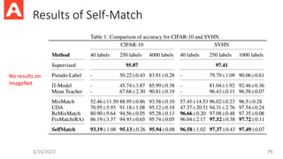
86. SSL Results and Results with different critics
3/16/2022 86
NegJSD and DotPr are bad,
NegL2 is slightly worse

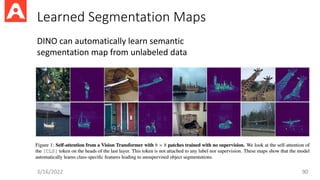
87. DINO
• Apply contrastive learning on a Vision Transformer (ViT)
• Verify the importance of momentum encoder, multi-crop training for
contrastive learning
• Achieve 78.3% Top 1 accuracy with the k-NN classifier, and 80.1% Top
1 accuracy with the linear classifier.
3/16/2022 87
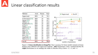
Better than supervised learning
with some ResNet architectures

88. Transformer
3/16/2022 88
Efficient Transformers: A Survey, Tay et al. 2020

89. Vision Transformer
3/16/2022 89
An Image Is Worth 16X16 Words: Transformers for Image Recognition at Scale, Dosovitskiy et al., 2020
An image is
converted into
a sequence of
patches
Simply reuse the
Transformer architecture

90. Learned Segmentation Maps
3/16/2022 90
DINO can automatically learn semantic
segmentation map from unlabeled data

91. Contrastive Learning for Unsupervised Domain
Adaptation
3/16/2022 91

92. Objective
• Assume labeled data from source domain and unlabeled data from
target domain. Adapt model to the target domain?
3/16/2022 92
Cross domain contrastive loss:
We need pseudo labels
from the target domain
Final objective:

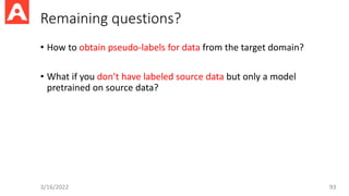
93. Remaining questions?
• How to obtain pseudo-labels for data from the target domain?
• What if you don’t have labeled source data but only a model
pretrained on source data?
3/16/2022 93

94. Results
3/16/2022 94

95. Contrastive Learning for Unsupervised Image-to-
Image Translation
3/16/2022 95

96. Results of CULIT
3/16/2022 96

97. Invariant Causal Mechanism (ReLIC)
3/16/2022 97

98. Objective of ReLIC
3/16/2022 98
Intervention on the style

99. 99
3/16/2022
Thank you for your attention!

100. 3/16/2022 100
Q&A