Isolation Forest
Fei Tony Liu, Zhi-Hua Zhou
Presenter: Jaehyeong Ahn
Department of Applied Statistics, Konkuk University
jayahn0104@gmail.com
1 / 1
Contents
Introduction
Basic Idea
Notation
Methodology
1 Training Stage
2 Evaluating Stage
Empirical Experiments
Summary
2 / 1
Introduction
• Anomalies are data patterns that have different data characteristics from
normal instances
• The detection of anomalies has significant relevance and often provides
critical actionable information in various application domains (e.g.
fraudulent use of credit cards, unusual computer network traffic pattern,
· · · )
• Most existing model-based approaches to anomaly detection construct a
profile of normal instances, then identify instances that do not conform to
the normal profile as anomalies
• However there are two major drawbacks of this approach
1 The anomaly detector is optimized to profile normal instances, but
not optimized to detect anomalies which causes too many false
alarms
2 Many existing methods are constrained to low dimensional data and
small data size because of their high computational complexity
3 / 1
Introduction
In this work,
• We introduce the method called ”Isolation Forest” or ”iForest” which is
suggested by [Liu et.al.]
• iForest proposes a different type of model-based method that explicitly
isolates anomalies rather than profiles normal instances
• iForest utilizes no distance or density measures to detect anomalies.
This eliminates major computational cost of distance calculation
• iForest has a linear time complexity with a low constant and a low
memory requirement
• iForest has the capacity to scale up to handle extremely large data
size and high-dimensional problems with a large number of
irrelevant attributes
• Assume:
1 Anomalies are the minority consisting of fewer instances
2 Anomalies have attribute-values that are very different from those
of normal instances
4 / 1
Basic Idea
• Construct an unsupervised decision tree which randomly partition the
sample space with binary split until every single instance is isolated. Call
this tree as iTree
• Because of their susceptibility to isolation, anomalies will be isolated
closer to the root of the tree; whereas normal points will be isolated at
the deeper end of the tree
• Build an iForest which is an ensemble of iTrees for sub-sampled,
bootstrapped without replacement, data sets
• Calculate the average path length of each data point and get anomaly
score by using some metric
• Identify data points as anomalies which have high anomaly score
5 / 1
Basic Idea
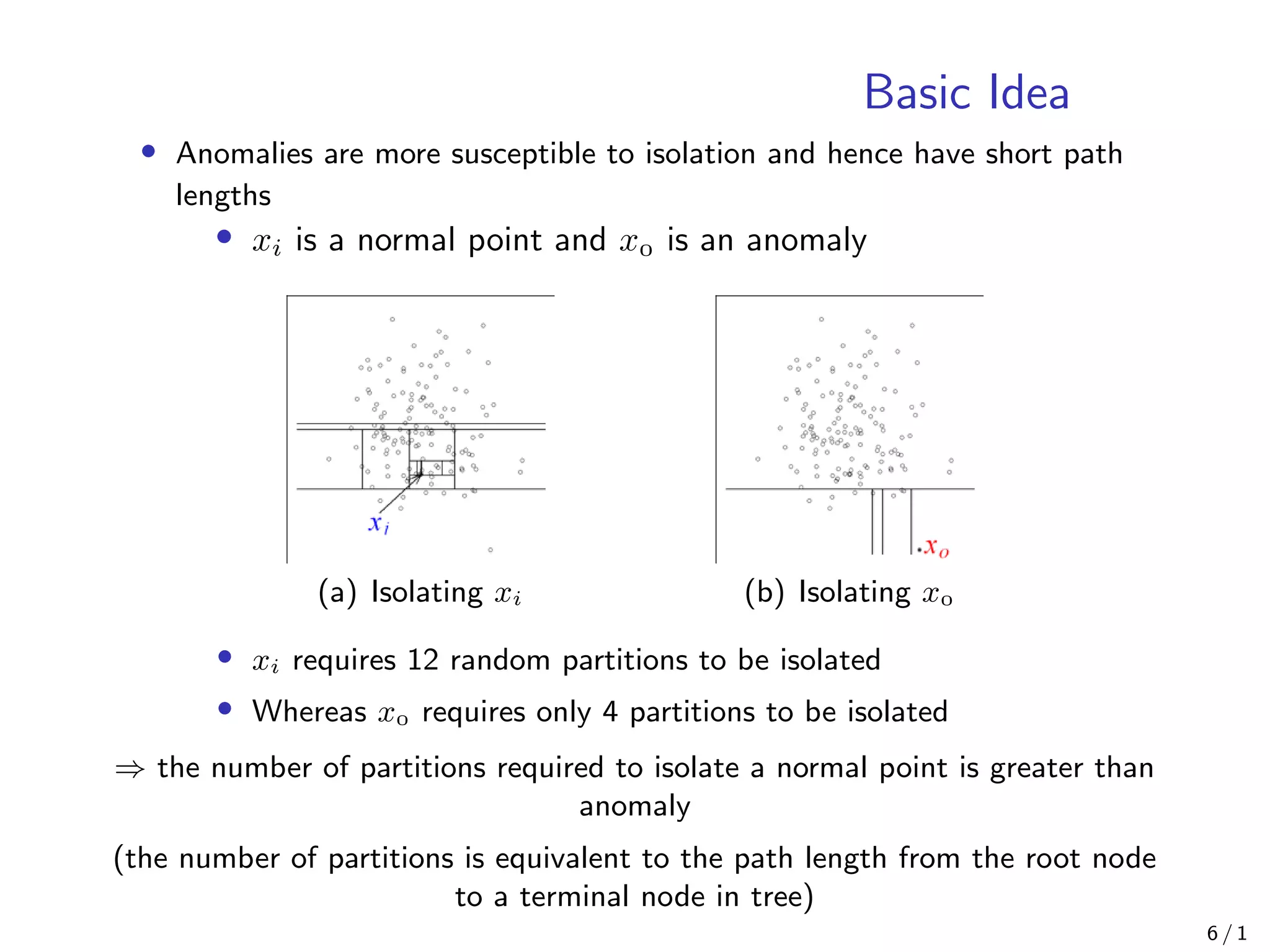
• Anomalies are more susceptible to isolation and hence have short path
lengths
• xi is a normal point and x is an anomaly
(a) Isolating xi (b) Isolating x
• xi requires 12 random partitions to be isolated
• Whereas x requires only 4 partitions to be isolated
⇒ the number of partitions required to isolate a normal point is greater than
anomaly
(the number of partitions is equivalent to the path length from the root node
to a terminal node in tree)
6 / 1
Basic Idea
Figure: Average path lengths converge
7 / 1
Notation
• X = {x, · · · , xn}, xi ∈ Rd
for all i = , · · · , N
• (only consider continuous valued attributes)
• T is a node of an isolation tree
• T is either an external-node (terminal-node) with no child, or an
internal-node with one test and exactly two daughter nodes (Tl, Tr)
• A test consists of an attribute q and a split value p such that the
test q < p divides data points into Tl and Tr
• h(x): Path Length of a point x which is measured by the number of
edges x traverses an iTree from the root node until the traversal is
terminated at an external node
• c(n): Average path length of unsuccessful search in BST(Binary Search
Tree)[B. R. Preiss,1999]. This is used for normalization of h(x),
(H(i) ≈ ln(i) + .)
c(n) = H(n − ) − ((n − )/n) (1)
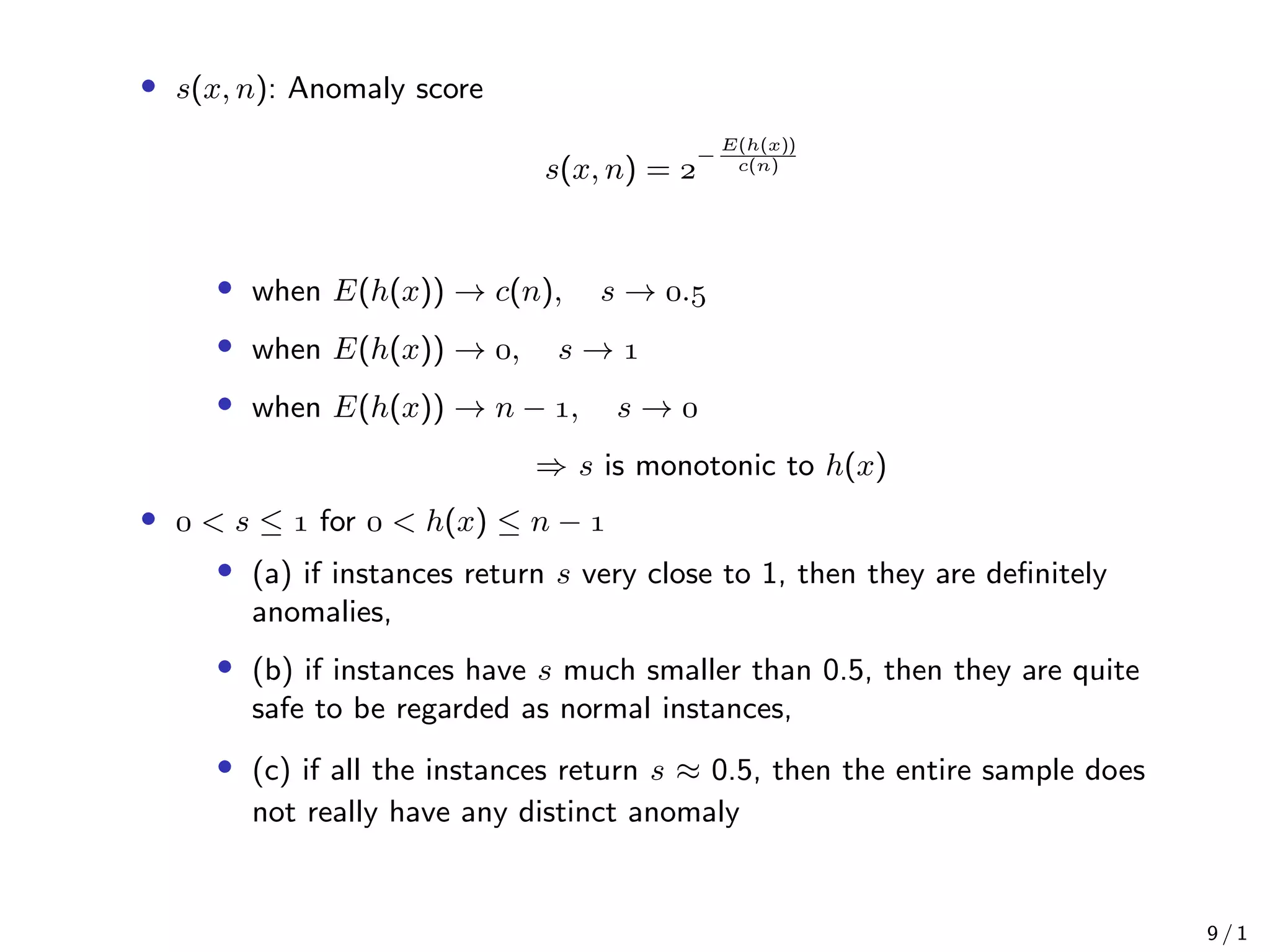
• s(x, n): Anomaly score
s(x, n) = 
−
E(h(x))
c(n) (2) 8 / 1
• s(x, n): Anomaly score
s(x, n) = 
−
E(h(x))
c(n)
• when E(h(x)) → c(n), s → .
• when E(h(x)) → , s → 
• when E(h(x)) → n − , s → 
⇒ s is monotonic to h(x)
•  < s ≤  for  < h(x) ≤ n − 
• (a) if instances return s very close to 1, then they are definitely
anomalies,
• (b) if instances have s much smaller than 0.5, then they are quite
safe to be regarded as normal instances,
• (c) if all the instances return s ≈ 0.5, then the entire sample does
not really have any distinct anomaly
9 / 1
Methodology
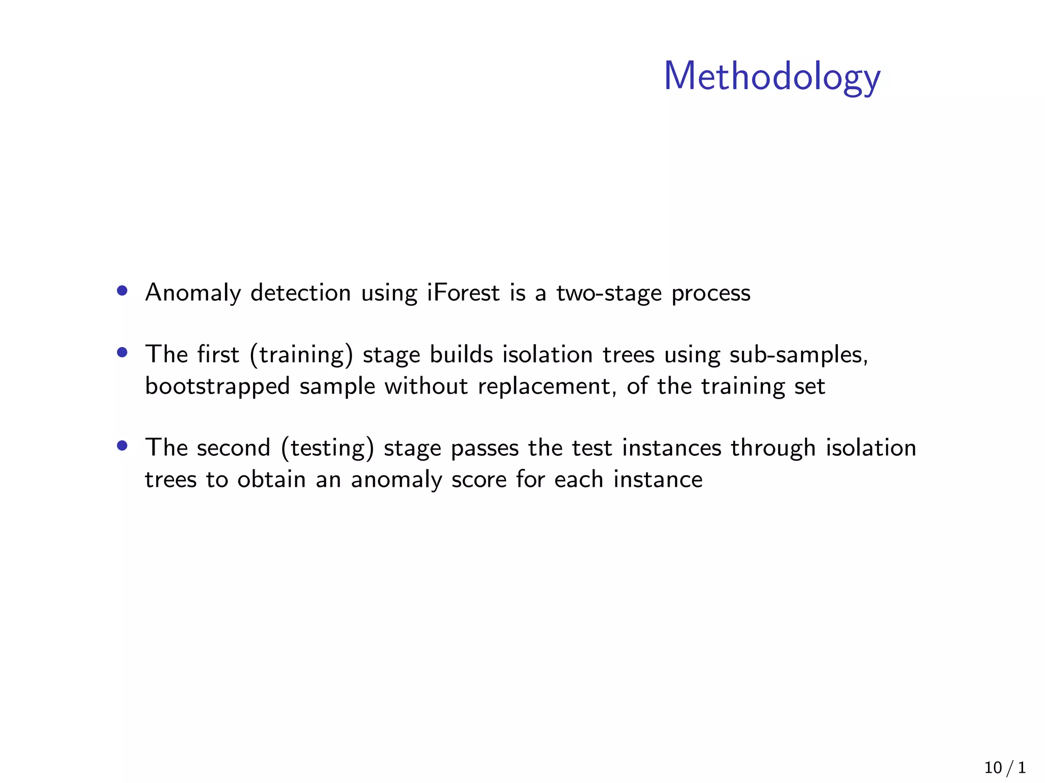
• Anomaly detection using iForest is a two-stage process
• The first (training) stage builds isolation trees using sub-samples,
bootstrapped sample without replacement, of the training set
• The second (testing) stage passes the test instances through isolation
trees to obtain an anomaly score for each instance
10 / 1
Training Stage
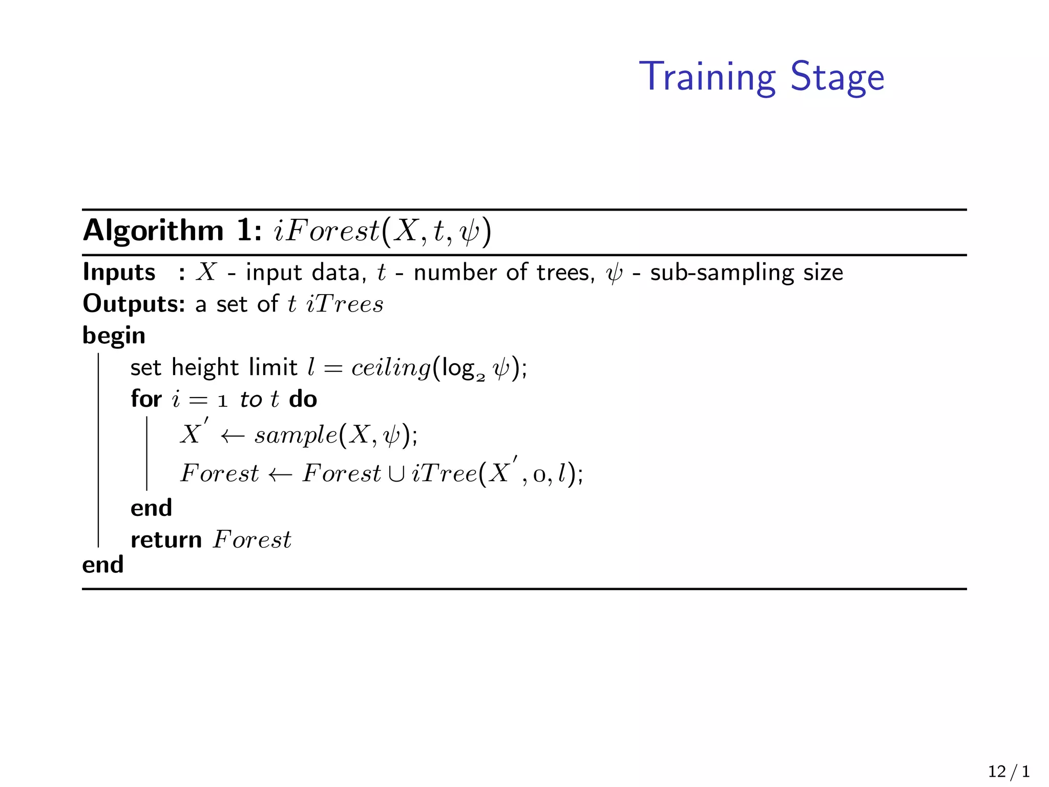
• In the training stage, iTrees are constructed by recursively partitioning the
given training set until instances are isolated or a specific tree height is
reached
• The tree height limit l is automatically set by the sub-sampling size
ψ : l = ceiling(log ψ) which is approximately the average tree height [D.
E. Knorr, 1998]
• The reason of setting a tree height limit is that we are only interested in
data points which have shorter than average path lengths, as those points
are more likely to be anomalies
• Details of the training stage can be found in following Algorithms 1 and 2
• The complexity of the training an iForest is O(tψ log ψ)
11 / 1
Training Stage
Algorithm 1: iForest(X, t, ψ)
Inputs : X - input data, t - number of trees, ψ - sub-sampling size
Outputs: a set of t iTrees
begin
set height limit l = ceiling(log ψ);
for i =  to t do
X ← sample(X, ψ);
Forest ← Forest ∪ iTree(X , , l);
end
return Forest
end
12 / 1
Training Stage
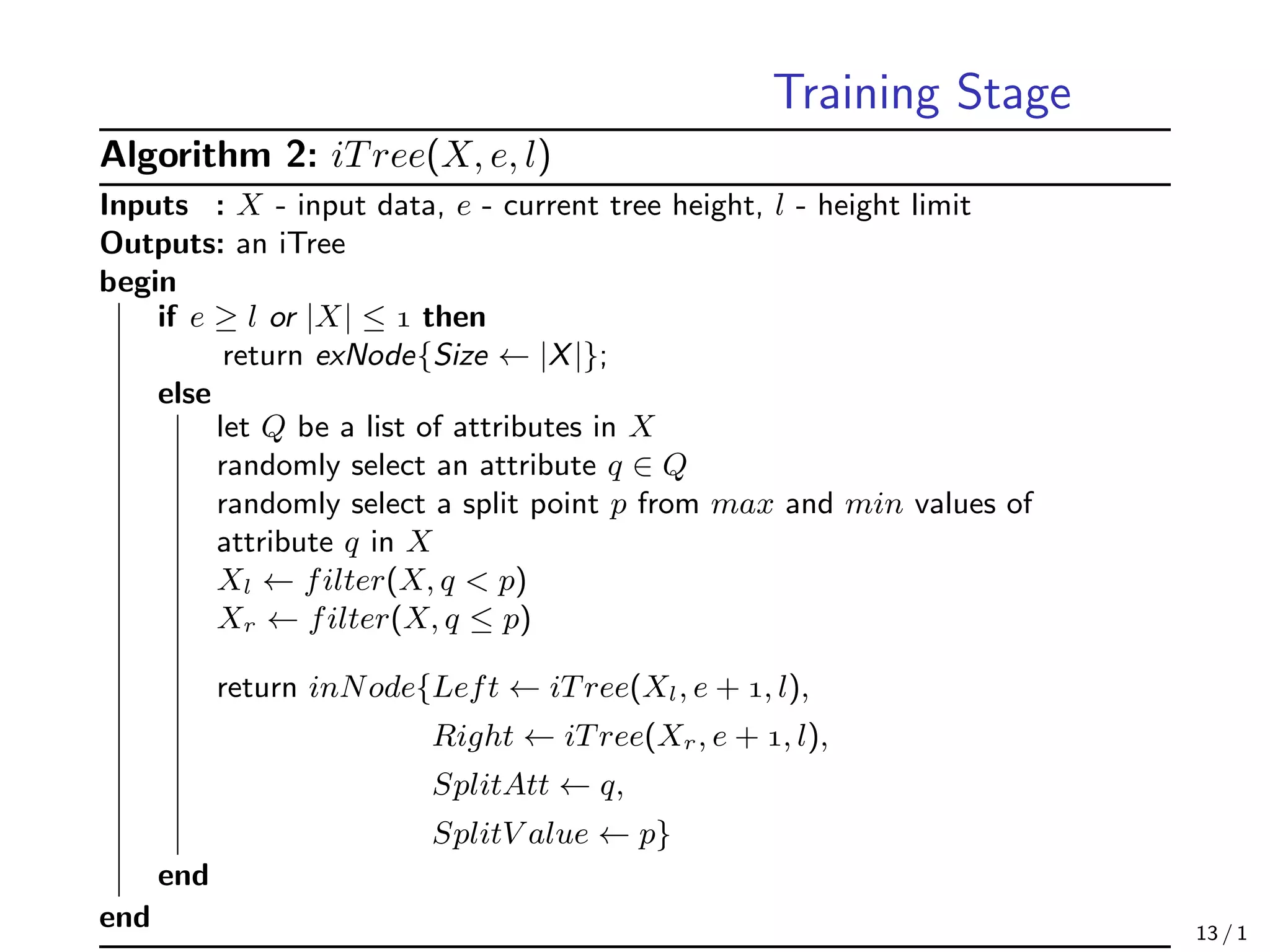
Algorithm 2: iTree(X, e, l)
Inputs : X - input data, e - current tree height, l - height limit
Outputs: an iTree
begin
if e ≥ l or |X| ≤  then
return exNode{Size ← |X|};
else
let Q be a list of attributes in X
randomly select an attribute q ∈ Q
randomly select a split point p from max and min values of
attribute q in X
Xl ← filter(X, q < p)
Xr ← filter(X, q ≤ p)
return inNode{Left ← iTree(Xl, e + , l),
Right ← iTree(Xr, e + , l),
SplitAtt ← q,
SplitV alue ← p}
end
end 13 / 1
Evaluating Stage
• In the evaluating stage, an anomaly score s is derived from the expected
path length E(h(x)) for each test instances
• E(h(x)) are derived by passing instances through each iTree in an iForest
• Using PathLength (Algorithm3) function, a single path length h(x) is
derived by counting the number of edges e from the root node to a
terminating node
• When h(x) is obtained for each tree of the ensemble, an anomaly score is
produced by computing s(x, ψ) in Equation 2
• To find the top m anomalies, simply sorts the data using s in descending
order. The first m instances are the top m anomalies
• The complexity of the evaluation process is O(nt log ψ), where n is the
testing data size
14 / 1
Evaluating Stage
Algorithm 3: PathLength(x, T, e)
Inputs : x - an instance, T - an iTree, e - current path length;
to be initialized to zero when first called
Outputs: path length of x
begin
if T is an external node then
return e + c(T.size){c(.)is defined in Equation 1}
end
a ← T.splitAtt;
if xa < T.splitV alue then
return PathLength(x, T.left, e + );
else if {xa ≥ T.splitV alue} then
return PathLength(x, T.right, e + )
end
end
15 / 1
Empirical Experiments
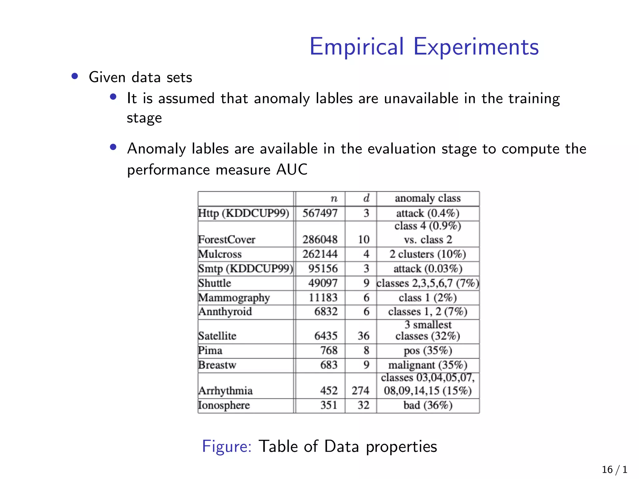
• Given data sets
• It is assumed that anomaly lables are unavailable in the training
stage
• Anomaly lables are available in the evaluation stage to compute the
performance measure AUC
Figure: Table of Data properties
16 / 1
Empirical Experiments
• Comparison with ORCA [Bay, 2003], LOF [Knox, 1998] and Random
Forests [Shi, 2006]
• For all the experiments, actual CPU time and Area Under Curve
(AUC) on ROC curve are reported as measurements
Figure: Table of Models
17 / 1
Empirical Experiments
• Early Convergence of AUC on iForest
• The performance of iForest is stable in wide range of t
• Since increasing t also increases processing time, the early
convergence of AUC suggests that iForest’s execution time can be
further reduces if t is tuned to a data set
(a) Arrhythmia (b) Satellite
Figure: Detection performance AUC (y-axis) is converged at a small t
(x-axis)
18 / 1
Empirical Experiments
• High Dimensional Data
• One of the important challenges in anomaly detection is high
dimensional data
• In this experiment, we study a special case in which high
dimensional data sets has a large number of irrelevant attributes or
background noises
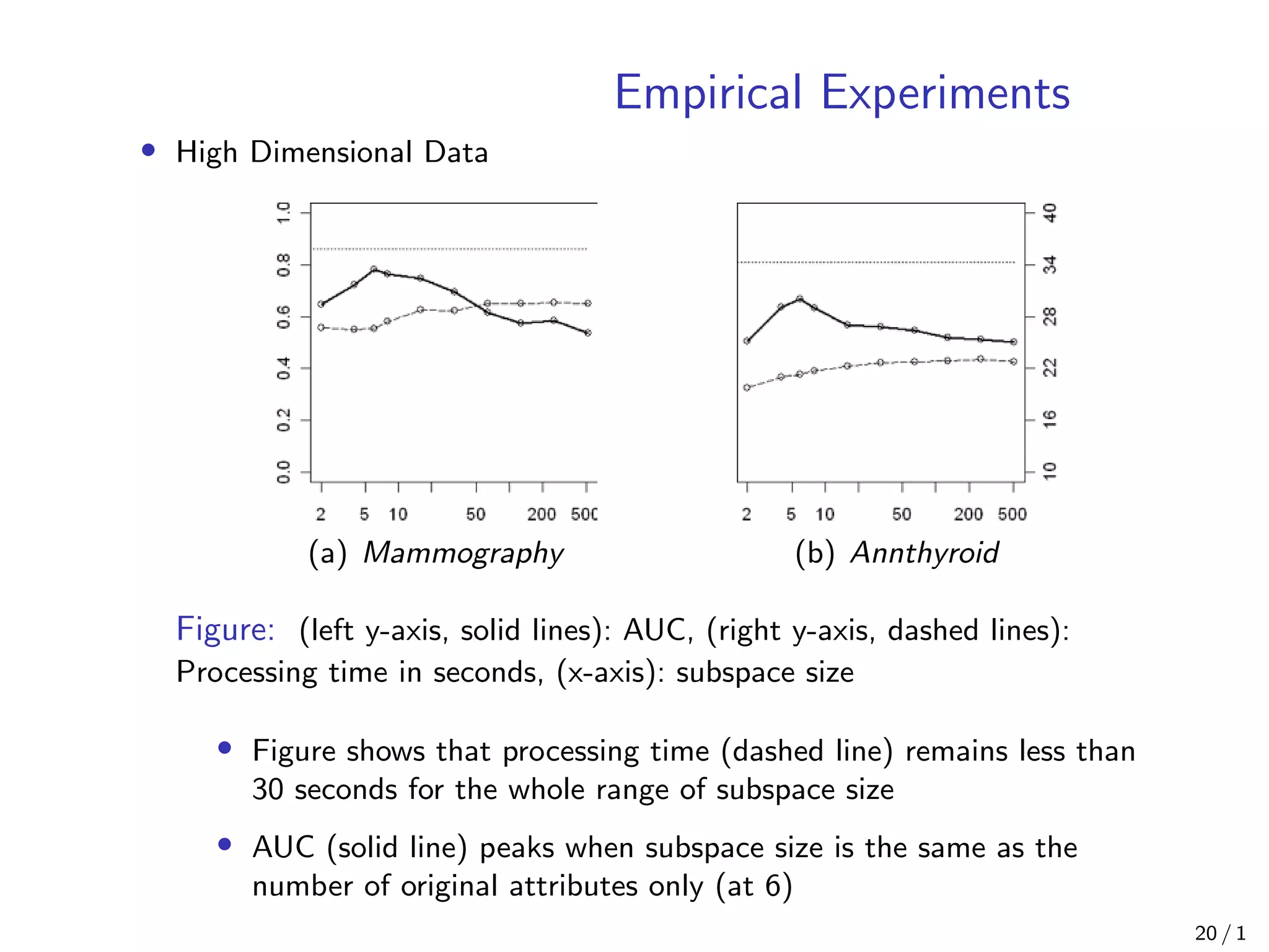
• Used data sets: Mammorgraphy (n=11183, d=6), Annthyroid
(n=6832, d=6)
• For each data set, 506 random variables added to simulate
background noise. Thus there is a total of 512 attributes in each
data sets
• We use a simple statistical test, Kurtosis, to select an attribute
subspace from the sub-sample before constructing each iTree
• After Kurtosis has provided a ranking for each attribute, a subspace
of attributes is selected according to this ranking to construct each
tree
19 / 1
Empirical Experiments
• High Dimensional Data
(a) Mammography (b) Annthyroid
Figure: (left y-axis, solid lines): AUC, (right y-axis, dashed lines):
Processing time in seconds, (x-axis): subspace size
• Figure shows that processing time (dashed line) remains less than
30 seconds for the whole range of subspace size
• AUC (solid line) peaks when subspace size is the same as the
number of original attributes only (at 6)
20 / 1
Summary
• In this work, we introduced a fundamentally different model-based
method that focuses on anomaly isolation rather than normal instance
profiling
• Taking advantage of anomalies’ nature of ’few and different’, iTree
isolates anomalies closer to the root of the tree as compared to normal
points
• This unique characteristic allows iForest to build partial models and
employ only a tiny proportion of training data to build effective models
• As a result, iForest has a linear time complexity with a low constant and
a low memory requiremnt which is ideal for high volume data sets
• Empirical experiments show that iForest out performs ORCA, LOF and
RF in terms of AUC and execution time, especially in large data sets
• Next works:
• Deal with categorical data
• Develop an elaborated random partition method
• Better dimension reduction (or variable selection) method
21 / 1
References
1 Liu, Fei Tony, Kai Ming Ting, and Zhi-Hua Zhou. ”Isolation forest.” In
2008 Eighth IEEE International Conference on Data Mining, pp. 413-422.
IEEE, 2008.
2 Preiss, Bruno R. ”Data Structures and Algorithms.” (1999).
3 Knuth, Donald E. ”The Art of Computer Programming, Volume 3:
Searching and Sorting.” Addison-Westley Publishing Company: Reading,
MA (1973).
4 Bay, Stephen D., and Mark Schwabacher. ”Mining distance-based outliers
in near linear time with randomization and a simple pruning rule.” In
Proceedings of the ninth ACM SIGKDD international conference on
Knowledge discovery and data mining, pp. 29-38. 2003.
5 Knox, Edwin M., and Raymond T. Ng. ”Algorithms for mining
distancebased outliers in large datasets.” In Proceedings of the
international conference on very large data bases, pp. 392-403. Citeseer,
1998.
6 Shi, Tao, and Steve Horvath. ”Unsupervised learning with random forest
predictors.” Journal of Computational and Graphical Statistics 15, no. 1
(2006): 118-138. 22 / 1

Isolation Forest

  • 1.
    Isolation Forest Fei TonyLiu, Zhi-Hua Zhou Presenter: Jaehyeong Ahn Department of Applied Statistics, Konkuk University jayahn0104@gmail.com 1 / 1
  • 2.
    Contents Introduction Basic Idea Notation Methodology 1 TrainingStage 2 Evaluating Stage Empirical Experiments Summary 2 / 1
  • 3.
    Introduction • Anomalies aredata patterns that have different data characteristics from normal instances • The detection of anomalies has significant relevance and often provides critical actionable information in various application domains (e.g. fraudulent use of credit cards, unusual computer network traffic pattern, · · · ) • Most existing model-based approaches to anomaly detection construct a profile of normal instances, then identify instances that do not conform to the normal profile as anomalies • However there are two major drawbacks of this approach 1 The anomaly detector is optimized to profile normal instances, but not optimized to detect anomalies which causes too many false alarms 2 Many existing methods are constrained to low dimensional data and small data size because of their high computational complexity 3 / 1
  • 4.
    Introduction In this work, •We introduce the method called ”Isolation Forest” or ”iForest” which is suggested by [Liu et.al.] • iForest proposes a different type of model-based method that explicitly isolates anomalies rather than profiles normal instances • iForest utilizes no distance or density measures to detect anomalies. This eliminates major computational cost of distance calculation • iForest has a linear time complexity with a low constant and a low memory requirement • iForest has the capacity to scale up to handle extremely large data size and high-dimensional problems with a large number of irrelevant attributes • Assume: 1 Anomalies are the minority consisting of fewer instances 2 Anomalies have attribute-values that are very different from those of normal instances 4 / 1
  • 5.
    Basic Idea • Constructan unsupervised decision tree which randomly partition the sample space with binary split until every single instance is isolated. Call this tree as iTree • Because of their susceptibility to isolation, anomalies will be isolated closer to the root of the tree; whereas normal points will be isolated at the deeper end of the tree • Build an iForest which is an ensemble of iTrees for sub-sampled, bootstrapped without replacement, data sets • Calculate the average path length of each data point and get anomaly score by using some metric • Identify data points as anomalies which have high anomaly score 5 / 1
  • 6.
    Basic Idea • Anomaliesare more susceptible to isolation and hence have short path lengths • xi is a normal point and x is an anomaly (a) Isolating xi (b) Isolating x • xi requires 12 random partitions to be isolated • Whereas x requires only 4 partitions to be isolated ⇒ the number of partitions required to isolate a normal point is greater than anomaly (the number of partitions is equivalent to the path length from the root node to a terminal node in tree) 6 / 1
  • 7.
    Basic Idea Figure: Averagepath lengths converge 7 / 1
  • 8.
    Notation • X ={x, · · · , xn}, xi ∈ Rd for all i = , · · · , N • (only consider continuous valued attributes) • T is a node of an isolation tree • T is either an external-node (terminal-node) with no child, or an internal-node with one test and exactly two daughter nodes (Tl, Tr) • A test consists of an attribute q and a split value p such that the test q < p divides data points into Tl and Tr • h(x): Path Length of a point x which is measured by the number of edges x traverses an iTree from the root node until the traversal is terminated at an external node • c(n): Average path length of unsuccessful search in BST(Binary Search Tree)[B. R. Preiss,1999]. This is used for normalization of h(x), (H(i) ≈ ln(i) + .) c(n) = H(n − ) − ((n − )/n) (1) • s(x, n): Anomaly score s(x, n) =  − E(h(x)) c(n) (2) 8 / 1
  • 9.
    • s(x, n):Anomaly score s(x, n) =  − E(h(x)) c(n) • when E(h(x)) → c(n), s → . • when E(h(x)) → , s →  • when E(h(x)) → n − , s →  ⇒ s is monotonic to h(x) •  < s ≤  for  < h(x) ≤ n −  • (a) if instances return s very close to 1, then they are definitely anomalies, • (b) if instances have s much smaller than 0.5, then they are quite safe to be regarded as normal instances, • (c) if all the instances return s ≈ 0.5, then the entire sample does not really have any distinct anomaly 9 / 1
  • 10.
    Methodology • Anomaly detectionusing iForest is a two-stage process • The first (training) stage builds isolation trees using sub-samples, bootstrapped sample without replacement, of the training set • The second (testing) stage passes the test instances through isolation trees to obtain an anomaly score for each instance 10 / 1
  • 11.
    Training Stage • Inthe training stage, iTrees are constructed by recursively partitioning the given training set until instances are isolated or a specific tree height is reached • The tree height limit l is automatically set by the sub-sampling size ψ : l = ceiling(log ψ) which is approximately the average tree height [D. E. Knorr, 1998] • The reason of setting a tree height limit is that we are only interested in data points which have shorter than average path lengths, as those points are more likely to be anomalies • Details of the training stage can be found in following Algorithms 1 and 2 • The complexity of the training an iForest is O(tψ log ψ) 11 / 1
  • 12.
    Training Stage Algorithm 1:iForest(X, t, ψ) Inputs : X - input data, t - number of trees, ψ - sub-sampling size Outputs: a set of t iTrees begin set height limit l = ceiling(log ψ); for i =  to t do X ← sample(X, ψ); Forest ← Forest ∪ iTree(X , , l); end return Forest end 12 / 1
  • 13.
    Training Stage Algorithm 2:iTree(X, e, l) Inputs : X - input data, e - current tree height, l - height limit Outputs: an iTree begin if e ≥ l or |X| ≤  then return exNode{Size ← |X|}; else let Q be a list of attributes in X randomly select an attribute q ∈ Q randomly select a split point p from max and min values of attribute q in X Xl ← filter(X, q < p) Xr ← filter(X, q ≤ p) return inNode{Left ← iTree(Xl, e + , l), Right ← iTree(Xr, e + , l), SplitAtt ← q, SplitV alue ← p} end end 13 / 1
  • 14.
    Evaluating Stage • Inthe evaluating stage, an anomaly score s is derived from the expected path length E(h(x)) for each test instances • E(h(x)) are derived by passing instances through each iTree in an iForest • Using PathLength (Algorithm3) function, a single path length h(x) is derived by counting the number of edges e from the root node to a terminating node • When h(x) is obtained for each tree of the ensemble, an anomaly score is produced by computing s(x, ψ) in Equation 2 • To find the top m anomalies, simply sorts the data using s in descending order. The first m instances are the top m anomalies • The complexity of the evaluation process is O(nt log ψ), where n is the testing data size 14 / 1
  • 15.
    Evaluating Stage Algorithm 3:PathLength(x, T, e) Inputs : x - an instance, T - an iTree, e - current path length; to be initialized to zero when first called Outputs: path length of x begin if T is an external node then return e + c(T.size){c(.)is defined in Equation 1} end a ← T.splitAtt; if xa < T.splitV alue then return PathLength(x, T.left, e + ); else if {xa ≥ T.splitV alue} then return PathLength(x, T.right, e + ) end end 15 / 1
  • 16.
    Empirical Experiments • Givendata sets • It is assumed that anomaly lables are unavailable in the training stage • Anomaly lables are available in the evaluation stage to compute the performance measure AUC Figure: Table of Data properties 16 / 1
  • 17.
    Empirical Experiments • Comparisonwith ORCA [Bay, 2003], LOF [Knox, 1998] and Random Forests [Shi, 2006] • For all the experiments, actual CPU time and Area Under Curve (AUC) on ROC curve are reported as measurements Figure: Table of Models 17 / 1
  • 18.
    Empirical Experiments • EarlyConvergence of AUC on iForest • The performance of iForest is stable in wide range of t • Since increasing t also increases processing time, the early convergence of AUC suggests that iForest’s execution time can be further reduces if t is tuned to a data set (a) Arrhythmia (b) Satellite Figure: Detection performance AUC (y-axis) is converged at a small t (x-axis) 18 / 1
  • 19.
    Empirical Experiments • HighDimensional Data • One of the important challenges in anomaly detection is high dimensional data • In this experiment, we study a special case in which high dimensional data sets has a large number of irrelevant attributes or background noises • Used data sets: Mammorgraphy (n=11183, d=6), Annthyroid (n=6832, d=6) • For each data set, 506 random variables added to simulate background noise. Thus there is a total of 512 attributes in each data sets • We use a simple statistical test, Kurtosis, to select an attribute subspace from the sub-sample before constructing each iTree • After Kurtosis has provided a ranking for each attribute, a subspace of attributes is selected according to this ranking to construct each tree 19 / 1
  • 20.
    Empirical Experiments • HighDimensional Data (a) Mammography (b) Annthyroid Figure: (left y-axis, solid lines): AUC, (right y-axis, dashed lines): Processing time in seconds, (x-axis): subspace size • Figure shows that processing time (dashed line) remains less than 30 seconds for the whole range of subspace size • AUC (solid line) peaks when subspace size is the same as the number of original attributes only (at 6) 20 / 1
  • 21.
    Summary • In thiswork, we introduced a fundamentally different model-based method that focuses on anomaly isolation rather than normal instance profiling • Taking advantage of anomalies’ nature of ’few and different’, iTree isolates anomalies closer to the root of the tree as compared to normal points • This unique characteristic allows iForest to build partial models and employ only a tiny proportion of training data to build effective models • As a result, iForest has a linear time complexity with a low constant and a low memory requiremnt which is ideal for high volume data sets • Empirical experiments show that iForest out performs ORCA, LOF and RF in terms of AUC and execution time, especially in large data sets • Next works: • Deal with categorical data • Develop an elaborated random partition method • Better dimension reduction (or variable selection) method 21 / 1
  • 22.
    References 1 Liu, FeiTony, Kai Ming Ting, and Zhi-Hua Zhou. ”Isolation forest.” In 2008 Eighth IEEE International Conference on Data Mining, pp. 413-422. IEEE, 2008. 2 Preiss, Bruno R. ”Data Structures and Algorithms.” (1999). 3 Knuth, Donald E. ”The Art of Computer Programming, Volume 3: Searching and Sorting.” Addison-Westley Publishing Company: Reading, MA (1973). 4 Bay, Stephen D., and Mark Schwabacher. ”Mining distance-based outliers in near linear time with randomization and a simple pruning rule.” In Proceedings of the ninth ACM SIGKDD international conference on Knowledge discovery and data mining, pp. 29-38. 2003. 5 Knox, Edwin M., and Raymond T. Ng. ”Algorithms for mining distancebased outliers in large datasets.” In Proceedings of the international conference on very large data bases, pp. 392-403. Citeseer, 1998. 6 Shi, Tao, and Steve Horvath. ”Unsupervised learning with random forest predictors.” Journal of Computational and Graphical Statistics 15, no. 1 (2006): 118-138. 22 / 1