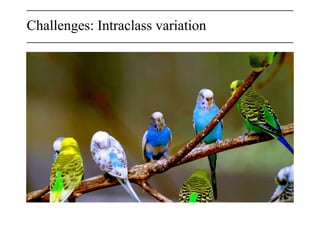
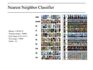
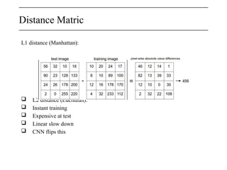
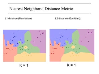
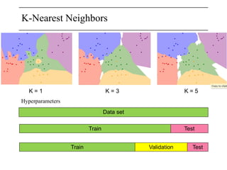
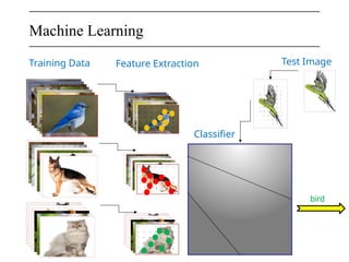
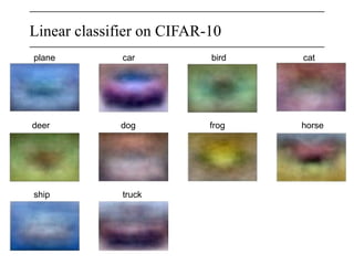
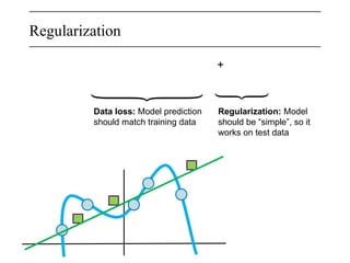
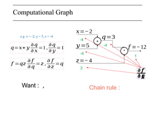
The document discusses neural networks, deep learning, and challenges related to them, with a focus on the CIFAR-10 dataset, which includes 50,000 training images. It details various classification techniques such as linear classifiers and softmax classifiers, and it emphasizes the importance of regularization and loss functions in machine learning. Additionally, it mentions the use of computational graphs and optimization methods for training neural networks.

1. Neural
Networks
By
Debajyoti Karmaker

2. 1
• Computer Science
2
• Artificial Intelligence
3
• Machine Learning
4
• Neural Networks
5
• Deep Learning
Hype about Deep Learning

3. Challenges: Semantic gap

4. Challenges: View point variation

5. Challenges: Deformation

6. Challenges: Occlusion

7. Challenges: background clutter

8. Challenges: Intraclass variation

9. Dataset : CIFAR-10
Training images : 50000
Each image is 32 x 32 x 3
Test images : 10000
Labels : 10
Nearest Neighbor Classifier

10. L1 distance (Manhattan):
 L2 distance (Euclidian):
 Instant training
 Expensive at test
 Linear slow down
 CNN flips this
Distance Matric

11. Nearest Neighbors: Distance Metric
L1 distance (Manhattan): L2 distance (Euclidian):

12. K-Nearest Neighbors
Hyperparameters
Data set
Train Test
Train Validation Test

13. Setting hyperparameters
Data set
Fold 1 Fold 2 Fold 3 Fold 4 Fold 5 test
Cross validation
Fold 1 Fold 2 Fold 3 Fold 4 Fold 5 test
Fold 1 Fold 2 Fold 3 Fold 4 Fold 5 test
Fold 1 Fold 2 Fold 3 Fold 4 Fold 5 test
Fold 1 Fold 2 Fold 3 Fold 4 Fold 5 test

14. Cross validation on CIFAR-10 dataset

15. Performance on CIFAR-10 (~29%)

16. Machine Learning
Training Data Feature Extraction Test Image
Classifier
bird

17. Linear Classification
[ 32 x 32 x 3 ] (3072 numbers in total)
10 numbers
Indicating class scores
¿𝑾 𝒙
Parametric approach
10
x
3072
3072
x
1
10
x
1
0.2 -0.5 0.1 2.0
1.5 1.3 2.1 0.0
0.0 0.25 0.2 -0.3
56
231
24
2
+
1.1
3.2
-1.2
-96.8
437.9
60.75
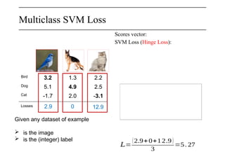
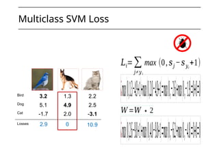
Bird score
Dog score
Cat score
𝑊
𝑥𝑖
𝑏 𝑓 (𝑥𝑖 ;𝑊 ,𝑏)
Stress pixels into single column
𝒇 (𝒙,𝑾 ) + b
56 231
24 2

18. Linear classifier on CIFAR-10
plane car bird cat
deer dog frog horse
ship truck

19. Multiclass SVM Loss
Scores vector:
SVM Loss (Hinge Loss):
Bird 3.2 1.3 2.2
Dog 5.1 4.9 2.5
Cat -1.7 2.0 -3.1
Losses 2.9 0 12.9
Given any dataset of example
 is the image
 is the (integer) label
𝐿=
(2.9+0+12.9 )
3
=5.27

20. Bird 3.2 1.3 2.2
Dog 5.1 4.9 2.5
Cat -1.7 2.0 -3.1
Losses 2.9 0 10.9
¿max(0,1.3−4.9+1)+max(0,2.0−4.9+1)=max(0,−2.6)+max(0,−1.9)=0+0=0
𝐿𝑖=∑
𝑗≠𝑦𝑖
max ⁡(0, 𝑠𝑗 −𝑠𝑦𝑖
+1)
Multiclass SVM Loss
¿max(0,2.6−9.8+1)+max(0,4.0−9.8+1)=max(0,−6.2)+max(0,−4.8)=0+0=0
𝑊=𝑊 ∗2

21. Regularization
Data loss: Model prediction
should match training data
Regularization: Model
should be “simple”, so it
works on test data
+

22. 𝐿=
1
𝑁
∑
𝑖=1
𝑁
∑
𝑗≠ 𝑦𝑖
max (0 , 𝑓 (𝑥𝑖 ,𝑊 )𝑗
− 𝑓 (𝑥𝑖 ,𝑊 )𝑦𝑖
+1)+ 𝜆 𝑅(𝑊 )
L2 regularization:
L1 regularization:
Elastic net (L2 + L1):
Model complexity: number of zeros
Model complexity: Smaller norm
Weight Regularization

23. 0.13
0.87
0.00
24.5
164.0
0.18
Softmax Classifier (Multinomial Logistic Regression)
scores = unnormalized log probabilities of the classes.
where
Bird 3.2
Dog 5.1
Cat -1.7
Want to maximize the log likelihood, or (for a loss function) to minimize the
negative log likelihood of the correct class:
)
𝐿𝑖=− log (
𝑒
𝑠𝑦 𝑖
∑
𝑗
𝑒𝑠𝑗
)⁡
exp normalize
unnormalized probabilities
unnormalized log probabilities probabilities

24. Optimization
A first very bad idea solution: Random search
15.5% accuracy! not bad! (SOTA is ~95%)

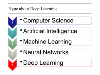
25. Numeric Gradient
Follow the slope
[
0.34
-1.11
0.78
0.12
0.55
2.81
-3.1
-1.5
0.33
… ]
[
0.34
-1.11
0.78
0.12
0.55
2.81
-3.1
-1.5
0.33
… ]
[
?
?
?
?
?
?
?
… ]
Current W W + h Gradient dW
+ 0.0001
+ 0.0001
loss 1.25347 loss 1.25322
?
?
-2.5
loss 1.25353
0.6

26. Computational Graph
e.g. x = -2, y = 5, z = -4
+
𝑥=−2
𝑦 =5
*
𝑞=3
𝑧=−4
𝑓 =−12
1
𝑞=𝑥+ 𝑦
𝜕𝑞
𝜕 𝑥
=1,
𝜕𝑞
𝜕 𝑦
=1
𝑓 =𝑞𝑧
𝜕 𝑓
𝜕𝑞
=𝑧 ,
𝜕 𝑓
𝜕𝑧
=𝑞
Want : ,
𝜕 𝑓
𝜕 𝑓
𝜕 𝑓
𝜕 𝑧
𝜕 𝑓
𝜕𝑞
3
𝜕 𝑓
𝜕 𝑦
-4
𝜕 𝑓
𝜕 𝑥
-4
Chain rule :
-4
Chain rule :

27. 𝑓 (𝑊 , 𝑥 )=
1
1+𝑒−(𝑤0 𝑥0+𝑤1 𝑥1 +𝑤2 )
Computational Graph
∗
∗
+¿ +¿ -1 𝑒𝑥𝑝
𝑤0
𝑥0
𝑤1
𝑥1
𝑤2
2.00
-1.00
-3.00
-2.00
-3.00
+1 1
𝑥
-2.00
6.00
4.00 1.00 -1.00 0.37 1.37 0.73
1.00
-0.53
-0.53
-0.20
0.20
0.20
0.20
0.20
0.20
-0.20
0.40
-0.40
-0.60 𝑓 (𝑥)=𝑒
𝑥
→
𝑑𝑓
𝑑𝑥
=𝑒
𝑥
𝑓 𝑐 (𝑥)=𝑐+𝑥 →
𝑑𝑓
𝑑𝑥
=1
𝑓 (𝑥)=
1
𝑥
→
𝑑𝑓
𝑑𝑥
=−
1
𝑥
2
𝑓 𝑎 (𝑥)=𝑎𝑥 →
𝑑𝑓
𝑑𝑥
=𝑎
(−
1
1.37
2 )∗(1.00 )=− 0.53
(1)(− 0.53)=− 0.53
(𝑒¿¿−1)(−0.53)=−0.20¿
(−1)(−0.20 )=0.20

28. ADD gate : Gradient distributor
Max gate : Gradient router
Mul gate: Gradient switcher
Patterns in backward flow

29. • Torch
• Theano
• Caffe
• Keras
• …
• etc
Deep Learning frameworks

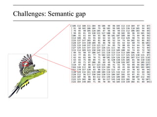
30. Vectorized example
∈ℝ𝑛
∈ℝ𝑛×𝑛
*
𝑊 =
[ 0 .1 0.5
− 0.3 0.8 ]
𝑥=[0 .2
0.4 ]
𝑞=𝑊.𝑥=
[𝑊1,1𝑥1+¿⋯ +𝑊1,𝑛𝑥𝑛
⋮ ¿
⋮¿𝑊𝑛,1𝑥1+¿⋯¿+𝑊𝑛,𝑛𝑥𝑛¿]
L2
[0 .2 2
0. 26 ] 0.116
1.00
[0 . 4 4
0. 52 ]
𝜕 𝑓
𝜕𝑞𝑖
=2𝑞𝑖
𝑓 (𝑞)
𝑞
𝜕𝑞𝑘
𝜕𝑊𝑖, 𝑗
=1𝑘=𝑖 𝑥 𝑗
𝑓 (𝑞)=‖𝑞‖
2
=𝑞1
2
+…+𝑞𝑛
2
[0 . 088 0. 104
0. 176 0. 208]
𝜕𝑞𝑘
𝜕 𝑥𝑖
=𝑊 𝑘,𝑖
[−0. 1 12
0.636 ]