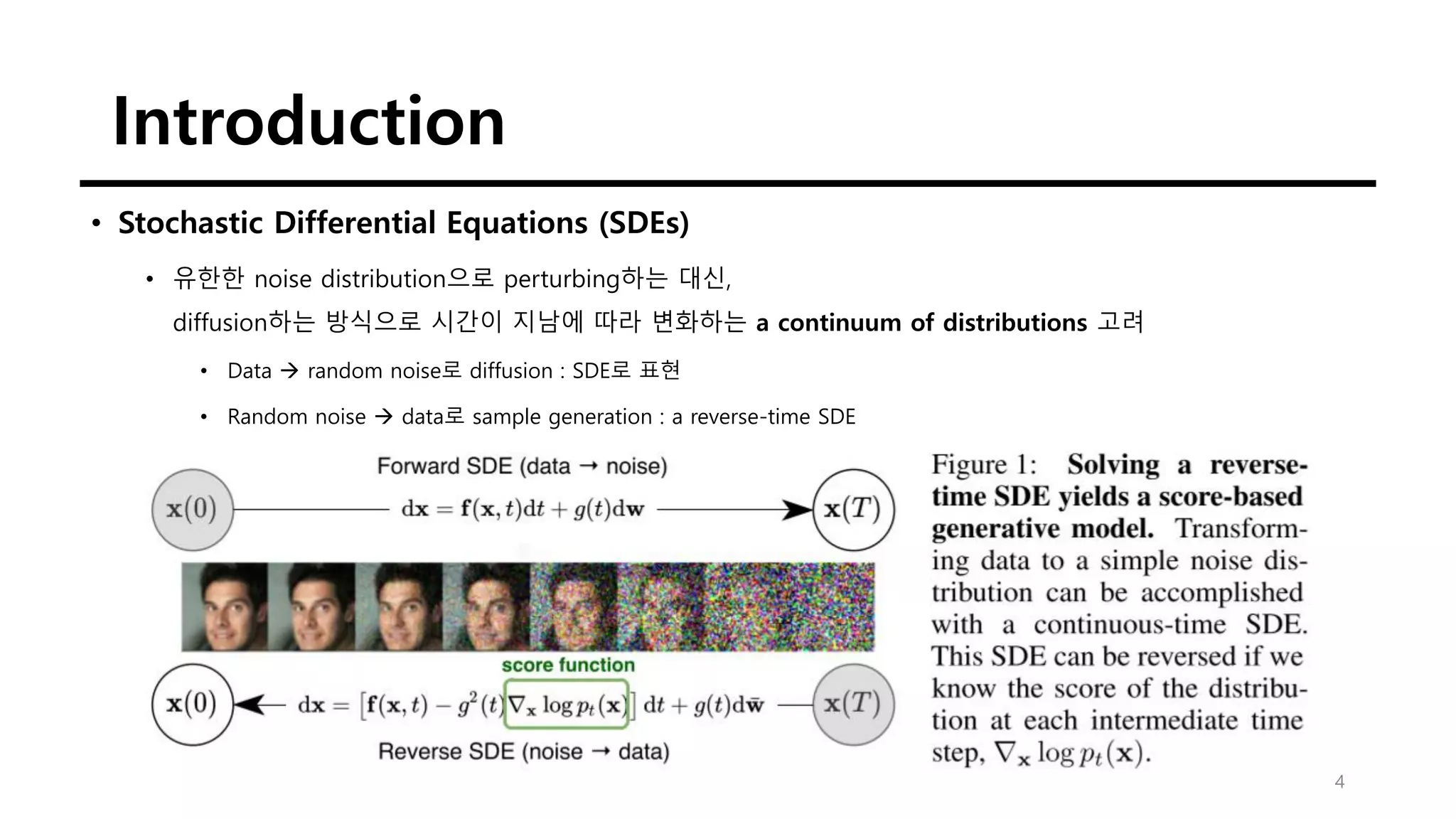
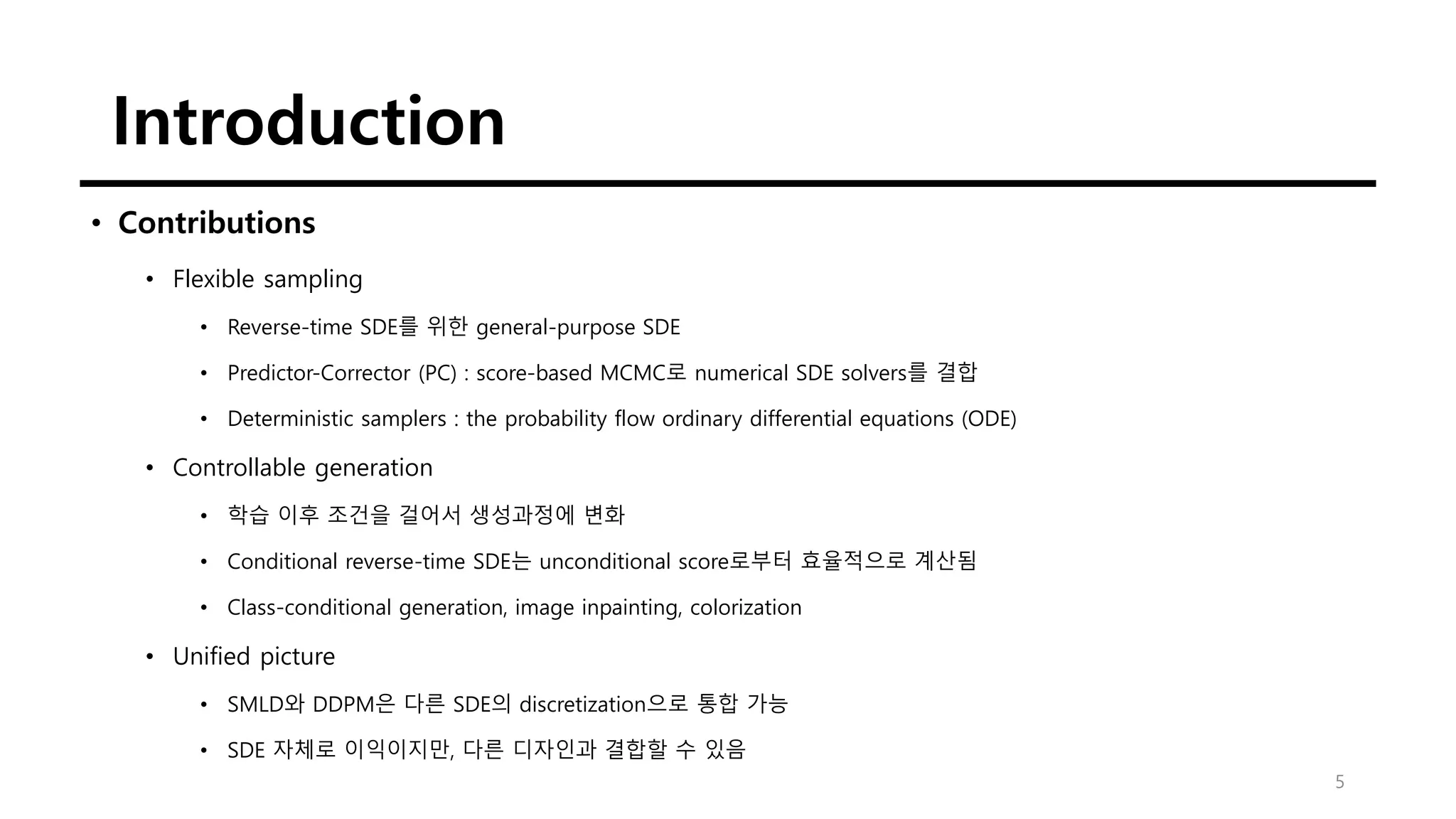
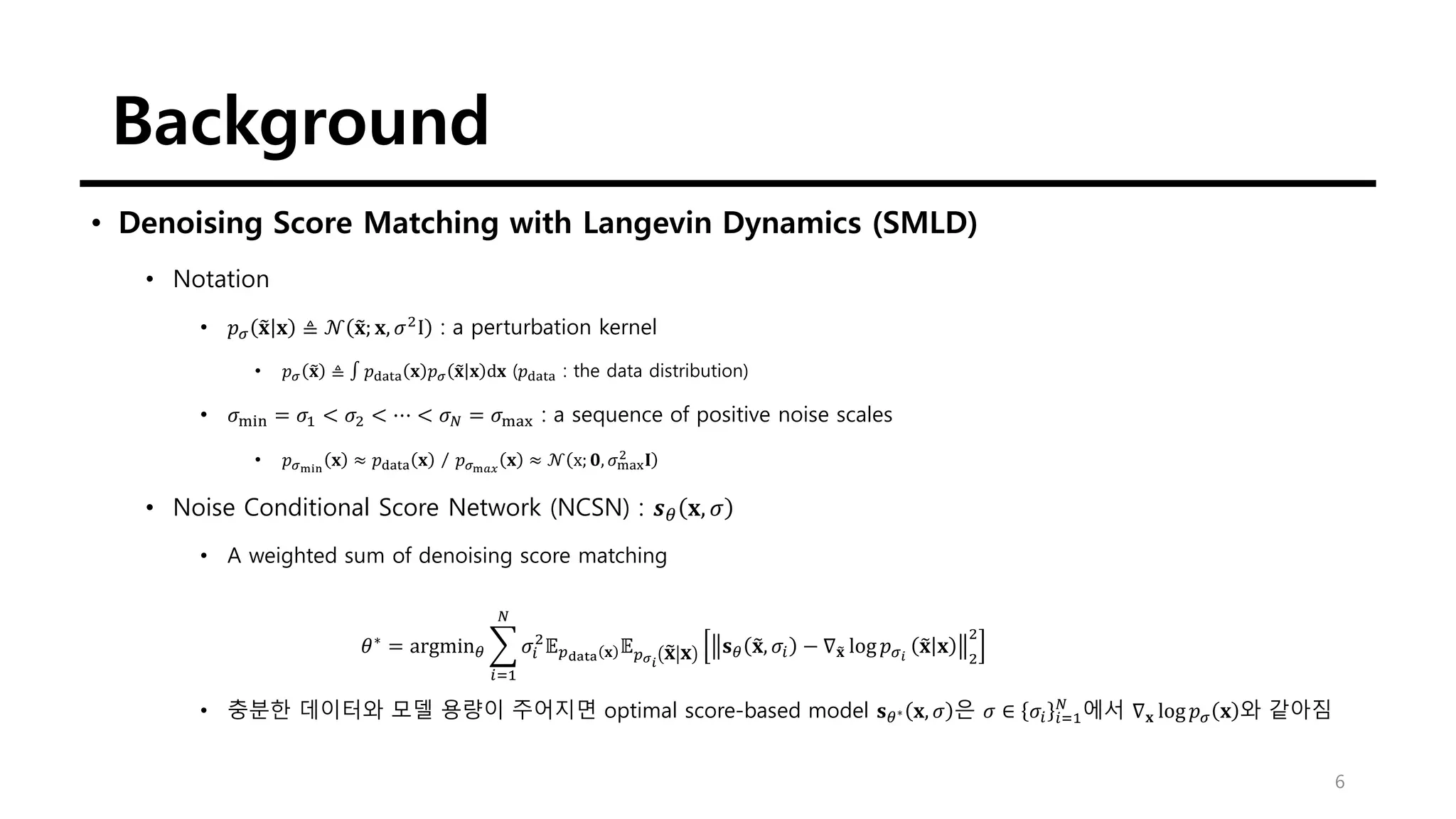
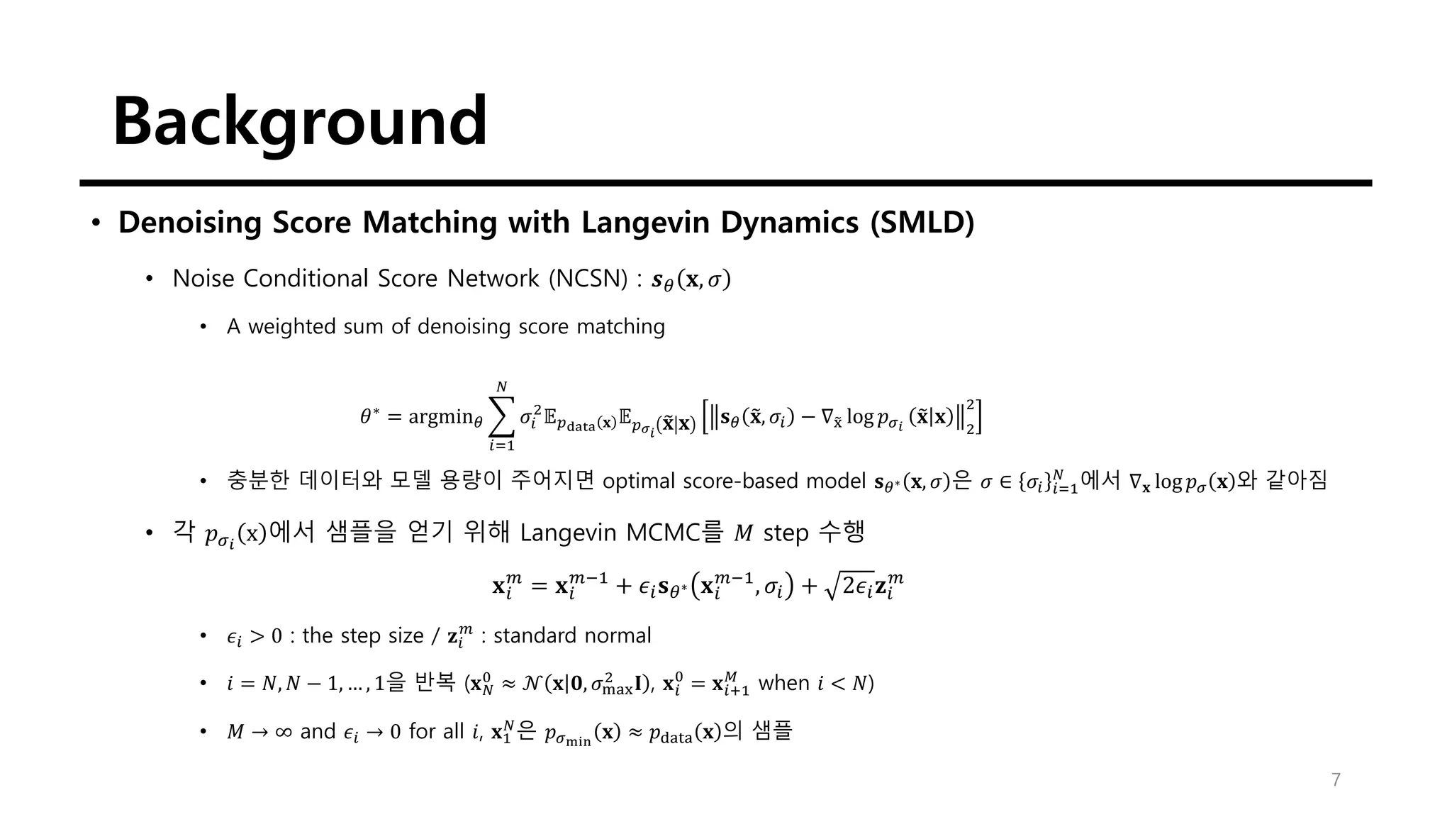
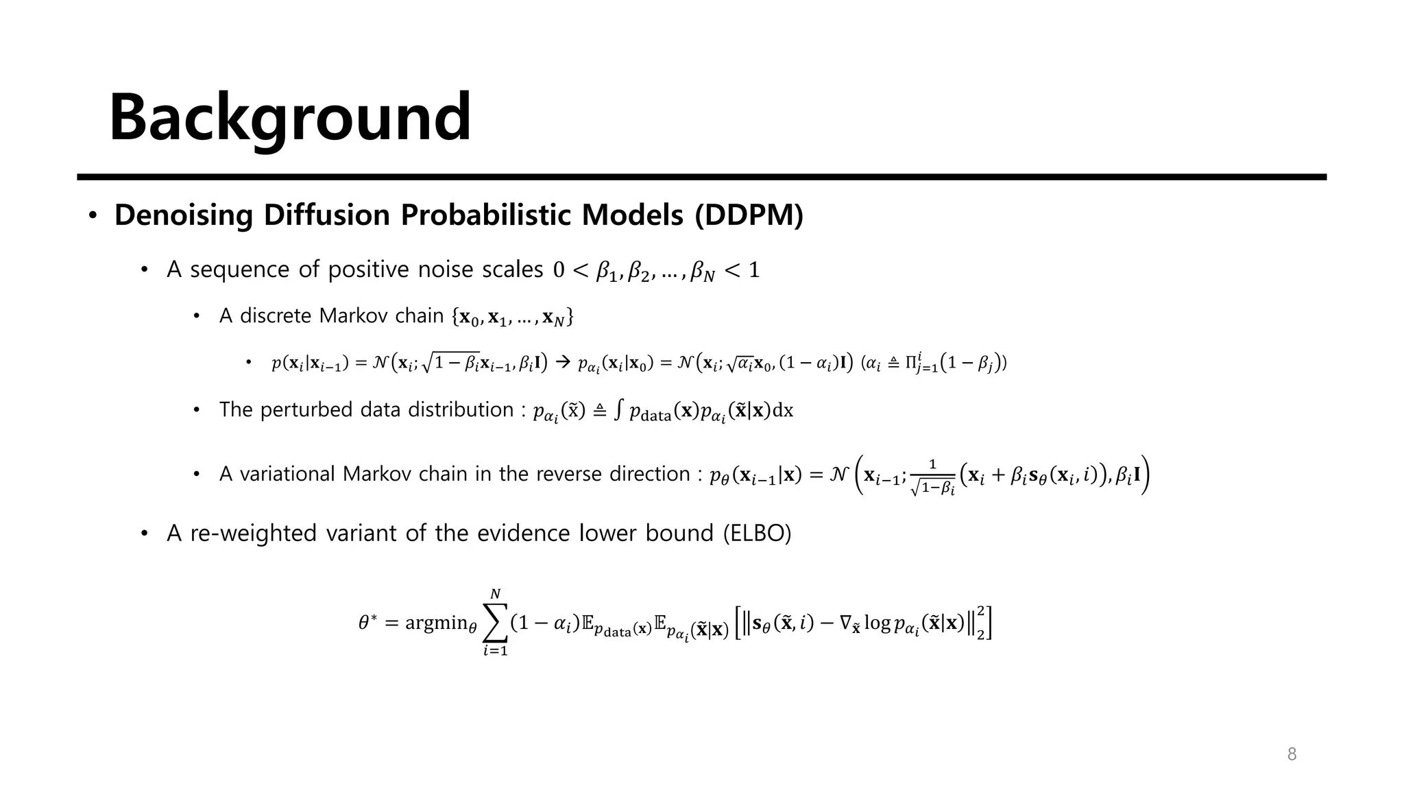
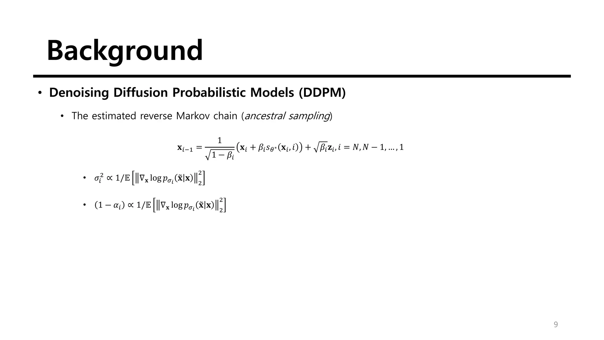
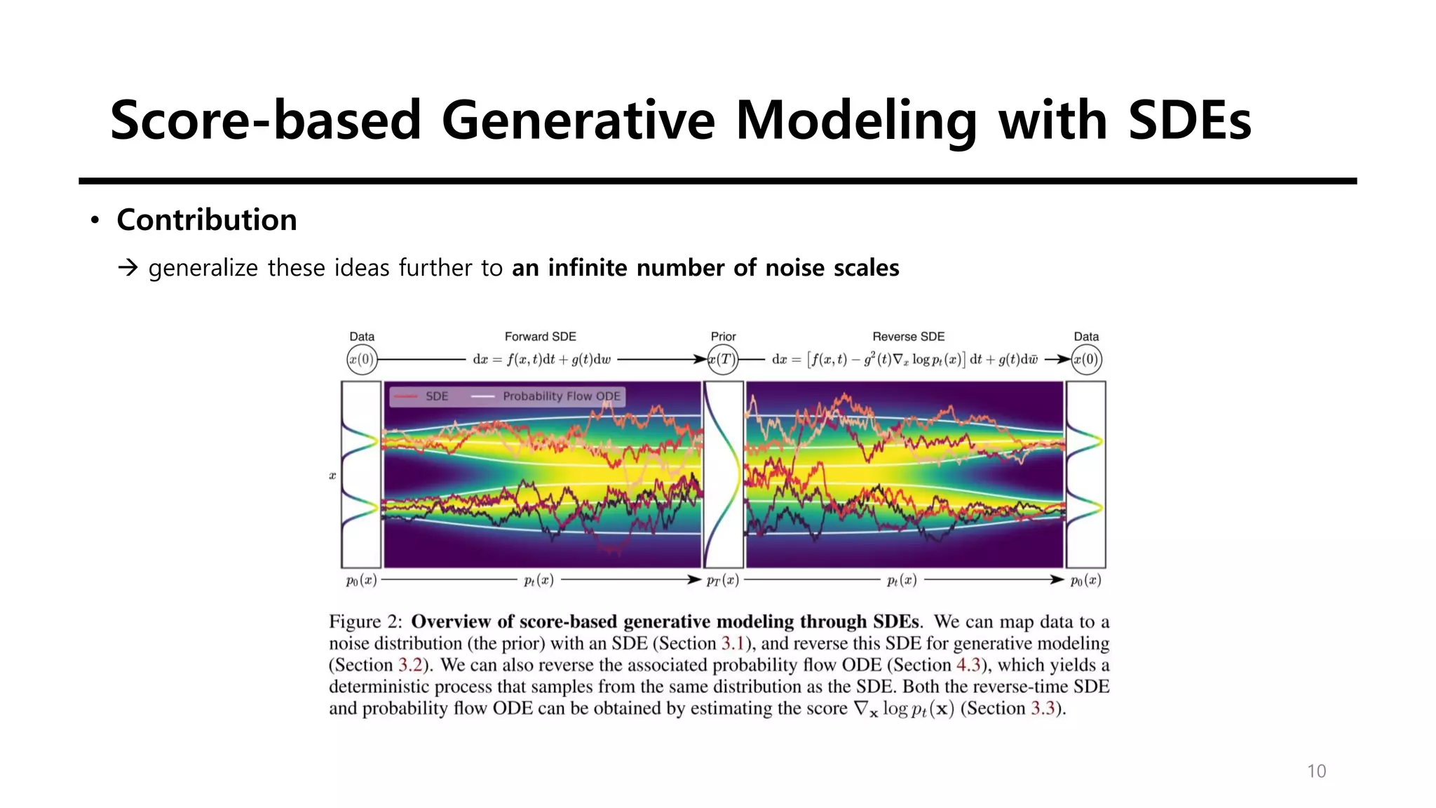
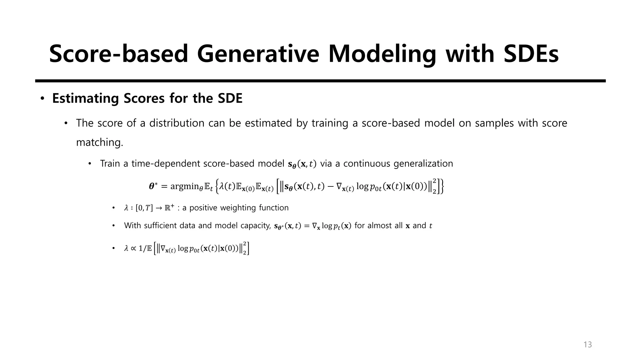
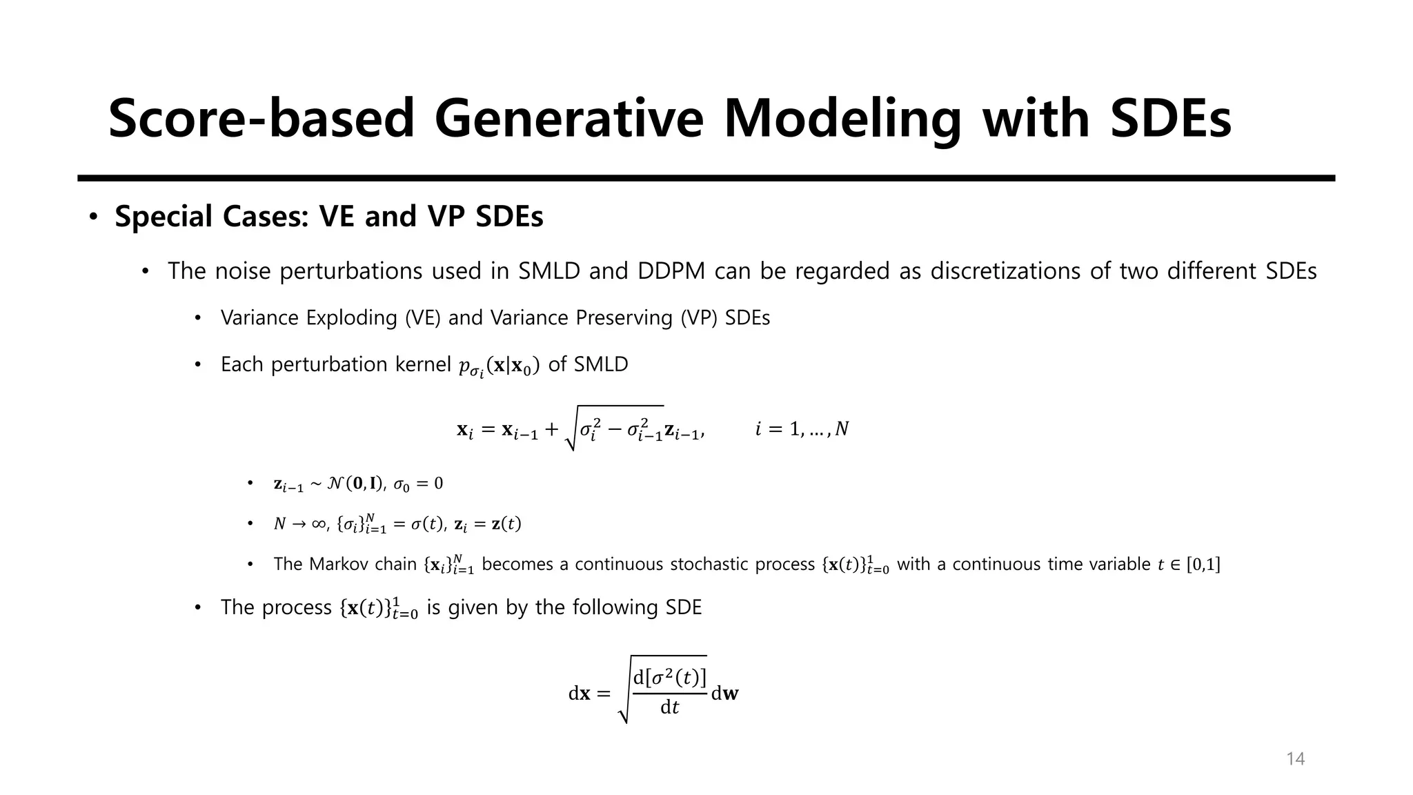
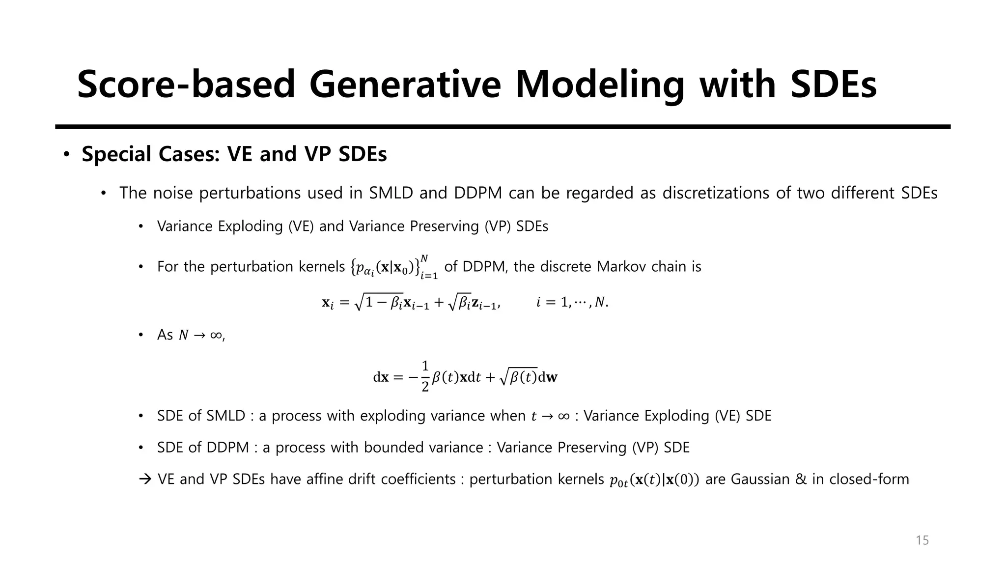
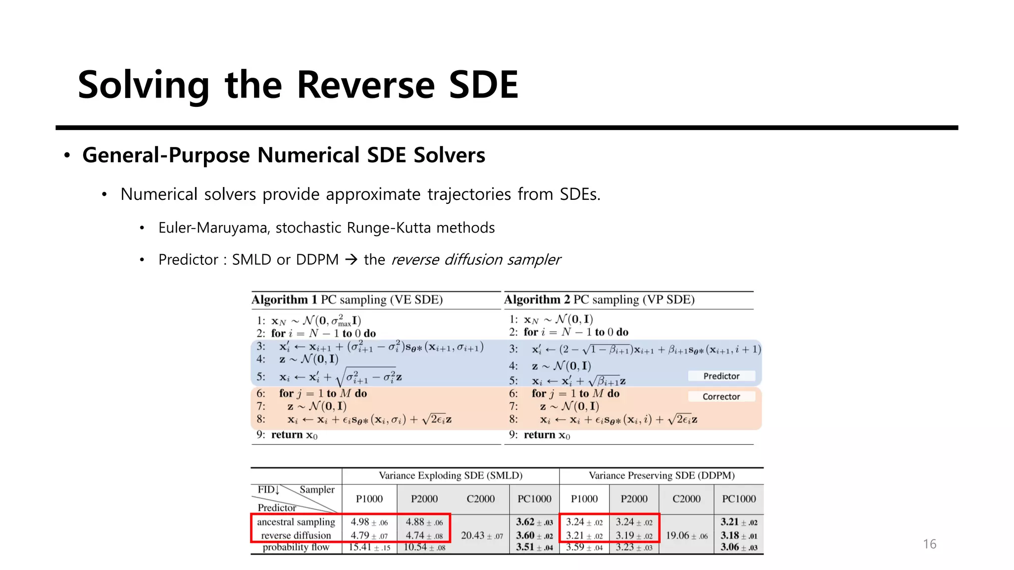
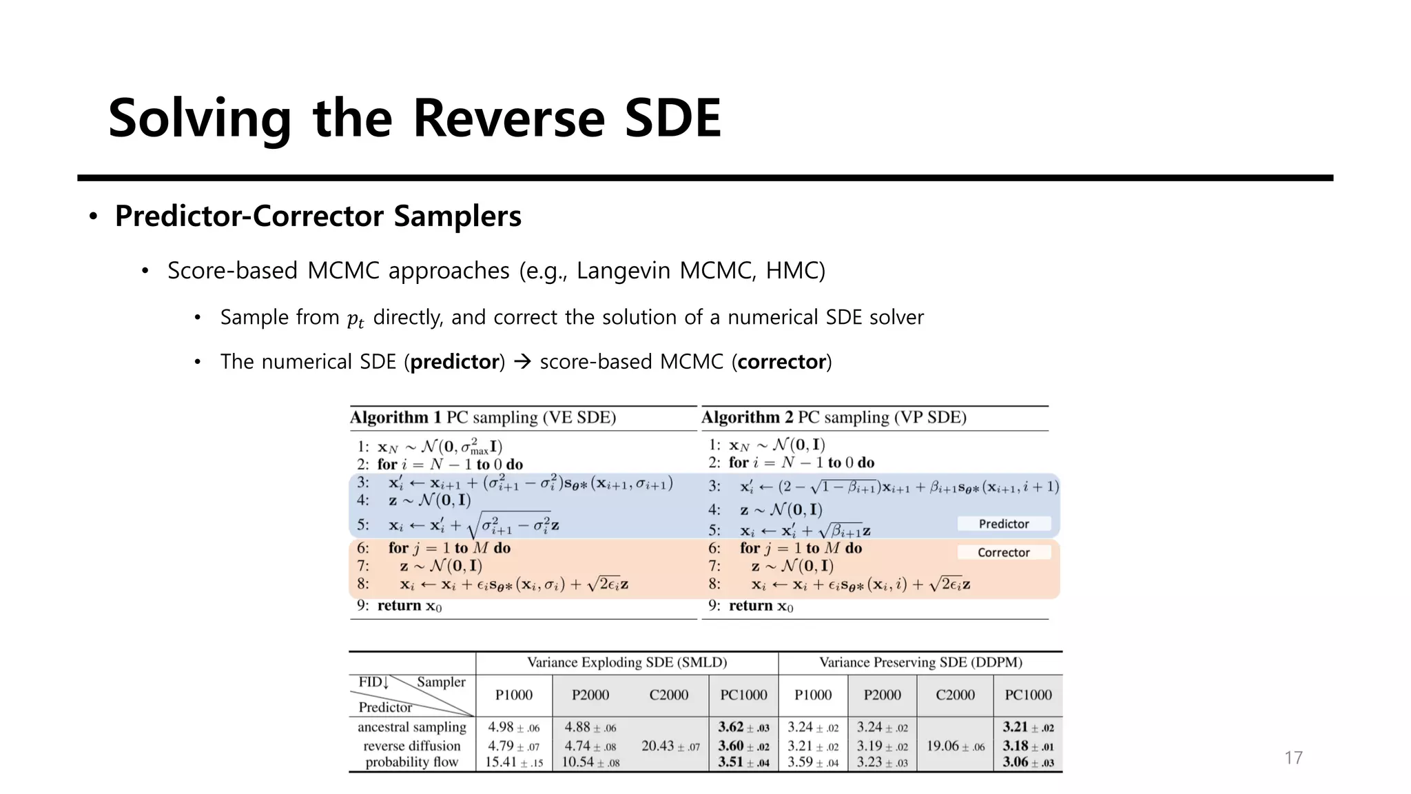
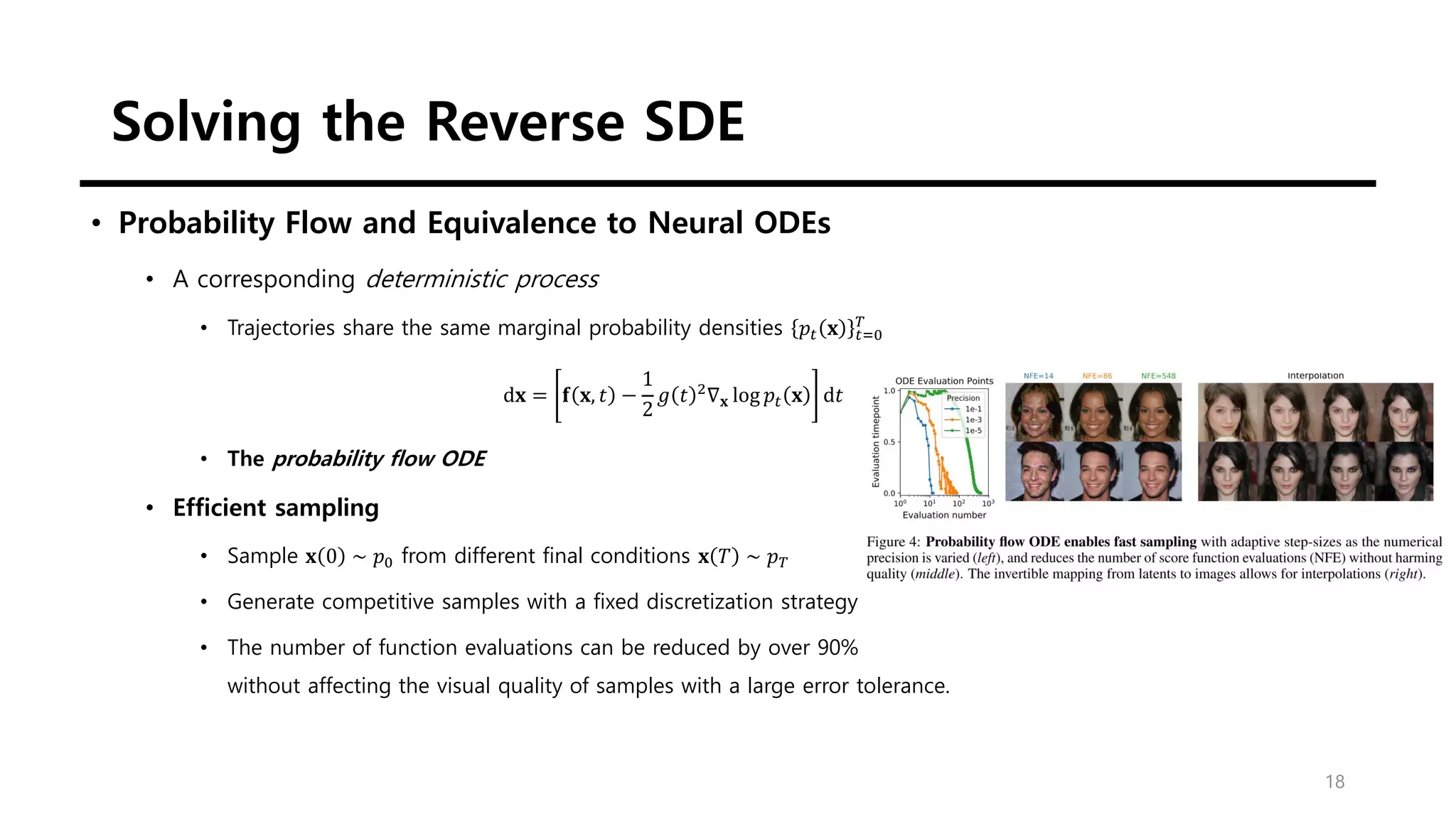
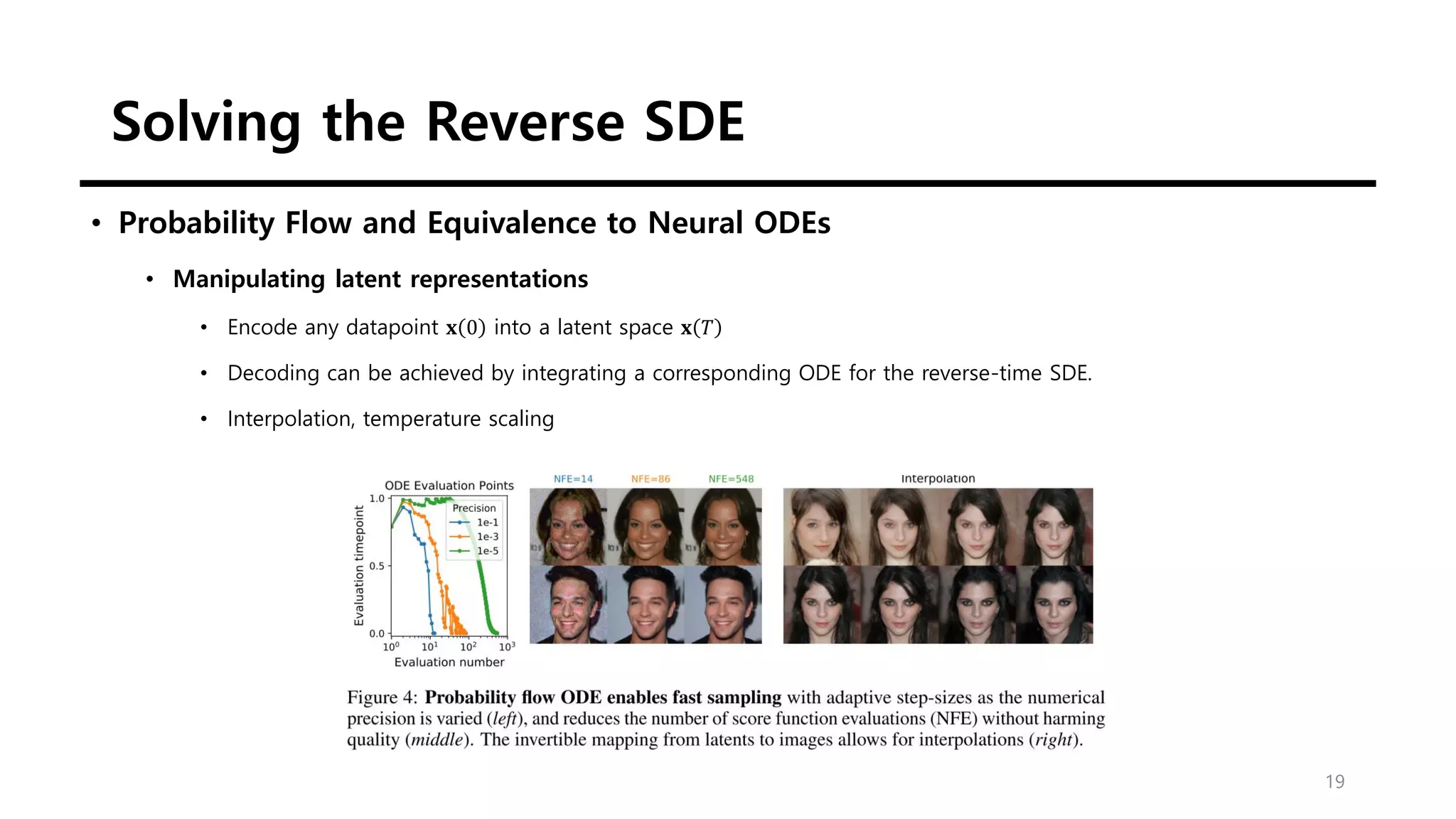
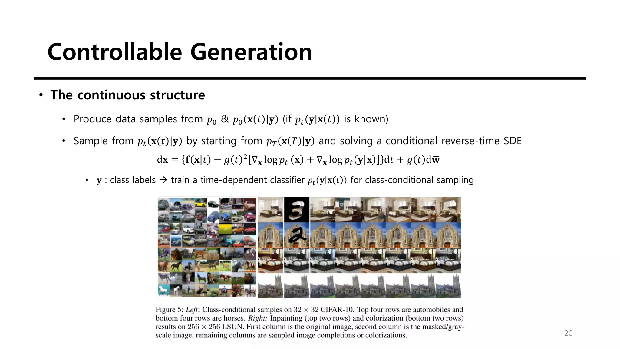
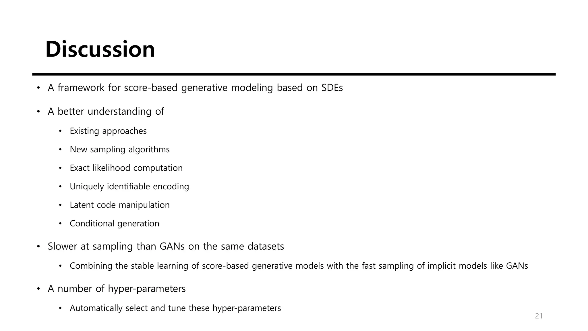
Sungchul Kim
Contents
1. Introduction
2. Background
3. Score-based generative modeling with SDEs
4. Solving the Reverse SDE
5. Controllable Generation
6. Discussion
2
Introduction
3
• Probabilistic generative models
• Slowly increasing noise / removing noise
• Score matching with Langevin dynamics (SMLD)
• 각 noise scale에서 score (i.e., the gradient of the log probability density, ∇𝐱log 𝑝𝑡 𝐱 ) 계산
• Noise scale 감소에 따른 샘플에 Langevin dynamics 적용
• Denoising diffusion probabilistic modeling (DDPM)
• Noise corruption을 거꾸로 하면서 학습
• 추적가능한 reverse distribution 사용
→ score-based generative models
• The practical performance of these two model classes is often quite different for reasons
that are not fully understood.
Introduction
4
• Stochastic Differential Equations (SDEs)
• 유한한 noise distribution으로 perturbing하는 대신,
diffusion하는 방식으로 시간이 지남에 따라 변화하는 a continuum of distributions 고려
• Data → random noise로 diffusion : SDE로 표현
• Random noise → data로 sample generation : a reverse-time SDE
Introduction
5
• Contributions
• Flexible sampling
• Reverse-time SDE를 위한 general-purpose SDE
• Predictor-Corrector (PC) : score-based MCMC로 numerical SDE solvers를 결합
• Deterministic samplers : the probability flow ordinary differential equations (ODE)
• Controllable generation
• 학습 이후 조건을 걸어서 생성과정에 변화
• Conditional reverse-time SDE는 unconditional score로부터 효율적으로 계산됨
• Class-conditional generation, image inpainting, colorization
• Unified picture
• SMLD와 DDPM은 다른 SDE의 discretization으로 통합 가능
• SDE 자체로 이익이지만, 다른 디자인과 결합할 수 있음
Background
6
• Denoising Score Matching with Langevin Dynamics (SMLD)
• Notation
• 𝑝𝜎 ෤
𝐱 𝐱 ≜ 𝒩 ෤
𝐱; 𝐱, 𝜎2
I : a perturbation kernel
• 𝑝𝜎 ෤
𝐱 ≜ ∫ 𝑝data 𝐱 𝑝𝜎 ෤
𝐱 𝐱 d𝐱 (𝑝data : the data distribution)
• 𝜎min = 𝜎1 < 𝜎2 < ⋯ < 𝜎𝑁 = 𝜎max : a sequence of positive noise scales
• 𝑝𝜎min
𝐱 ≈ 𝑝data 𝐱 / 𝑝𝜎m𝑎𝑥
𝐱 ≈ 𝒩 x; 𝟎, 𝜎max
2
𝐈
• Noise Conditional Score Network (NCSN) : 𝒔𝜃 𝐱, 𝜎
• A weighted sum of denoising score matching
𝜃∗
= argmin𝜃 ෍
𝑖=1
𝑁
𝜎𝑖
2
𝔼𝑝data 𝐱 𝔼𝑝𝜎𝑖
෤
𝐱 𝐱 𝐬𝜃 ෤
𝐱, 𝜎𝑖 − ∇෤
𝐱 log𝑝𝜎𝑖
෤
𝐱 𝐱
2
2
• 충분한 데이터와 모델 용량이 주어지면 optimal score-based model 𝐬𝜃∗ 𝐱, 𝜎 은 𝜎 ∈ 𝜎𝑖 𝑖=1
𝑁
에서 ∇𝐱 log𝑝𝜎 𝐱 와 같아짐
Background
7
• Denoising Score Matching with Langevin Dynamics (SMLD)
• Noise Conditional Score Network (NCSN) : 𝒔𝜃 𝐱, 𝜎
• A weighted sum of denoising score matching
𝜃∗
= argmin𝜃 ෍
𝑖=1
𝑁
𝜎𝑖
2
𝔼𝑝data 𝐱 𝔼𝑝𝜎𝑖
෤
𝐱 𝐱 𝐬𝜃 ෤
𝐱, 𝜎𝑖 − ∇෤
x log 𝑝𝜎𝑖
෤
𝐱 𝐱
2
2
• 충분한 데이터와 모델 용량이 주어지면 optimal score-based model 𝐬𝜃∗ 𝐱, 𝜎 은 𝜎 ∈ 𝜎𝑖 𝑖=1
𝑁
에서 ∇𝐱 log𝑝𝜎 𝐱 와 같아짐
• 각 𝑝𝜎𝑖
x 에서 샘플을 얻기 위해 Langevin MCMC를 𝑀 step 수행
𝐱𝑖
𝑚
= 𝐱𝑖
𝑚−1
+ 𝜖𝑖𝐬𝜃∗ 𝐱𝑖
𝑚−1
, 𝜎𝑖 + 2𝜖𝑖𝐳𝑖
𝑚
• 𝜖𝑖 > 0 : the step size / 𝐳𝑖
𝑚
: standard normal
• 𝑖 = 𝑁, 𝑁 − 1, … , 1을 반복 (𝐱𝑁
0
≈ 𝒩 𝐱 𝟎, 𝜎max
2
𝐈 , 𝐱𝑖
0
= 𝐱𝑖+1
𝑀
when 𝑖 < 𝑁)
• 𝑀 → ∞ and 𝜖𝑖 → 0 for all 𝑖, 𝐱1
𝑁
은 𝑝𝜎min
𝐱 ≈ 𝑝data 𝐱 의 샘플
Background
8
• Denoising Diffusion Probabilistic Models (DDPM)
• A sequence of positive noise scales 0 < 𝛽1, 𝛽2, … , 𝛽𝑁 < 1
• A discrete Markov chain 𝐱0, 𝐱1, … , 𝐱𝑁
• 𝑝 𝐱𝑖 𝐱𝑖−1 = 𝒩 𝐱𝑖; 1 − 𝛽𝑖𝐱𝑖−1, 𝛽𝑖𝐈 → 𝑝𝛼𝑖
𝐱𝑖 𝐱0 = 𝒩 𝐱𝑖; 𝛼𝑖𝐱0, 1 − 𝛼𝑖 𝐈 (𝛼𝑖 ≜ Π𝑗=1
𝑖
1 − 𝛽𝑗 )
• The perturbed data distribution : 𝑝𝛼𝑖
෤
x ≜ ∫ 𝑝data 𝐱 𝑝𝛼𝑖
෤
𝐱 𝐱 dx
• A variational Markov chain in the reverse direction : 𝑝𝜃 𝐱𝑖−1 𝐱 = 𝒩 𝐱𝑖−1;
1
1−𝛽𝑖
𝐱𝑖 + 𝛽𝑖𝐬𝜃 𝐱𝑖, 𝑖 , 𝛽𝑖𝐈
• A re-weighted variant of the evidence lower bound (ELBO)
𝜃∗
= argmin𝜃 ෍
𝑖=1
𝑁
1 − 𝛼𝑖 𝔼𝑝data 𝐱 𝔼𝑝𝛼𝑖
෤
𝐱 𝐱 𝐬𝜃 ෤
𝐱, 𝑖 − ∇෤
𝐱 log 𝑝𝛼𝑖
෤
𝐱 𝐱
2
2
Background
9
• Denoising Diffusion Probabilistic Models (DDPM)
• The estimated reverse Markov chain (ancestral sampling)
𝐱𝑖−1 =
1
1 − 𝛽𝑖
𝐱𝑖 + 𝛽𝑖𝑠𝜃∗ 𝐱𝑖, 𝑖 + 𝛽𝑖𝐳𝑖, 𝑖 = 𝑁, 𝑁 − 1, … , 1
• 𝜎𝑖
2
∝ 1/𝔼 ∇𝐱 log 𝑝𝜎𝑖
෤
𝐱 𝐱
2
2
• 1 − 𝛼𝑖 ∝ 1/𝔼 ∇𝐱 log𝑝𝜎𝑖
෤
𝐱 𝐱
2
2
Score-based Generative Modeling with SDEs
10
• Contribution
→ generalize these ideas further to an infinite number of noise scales
Score-based Generative Modeling with SDEs
11
• Perturbing Data with SDEs
• 목표 : a diffusion process 𝐱 𝑡 𝑡=0
𝑇
indexed by a continuous time variable 𝑡 ∈ 0, 𝑇
• x 0 ∼ 𝑝0 for which we have a dataset of i.i.d. samples (𝑝0 : the data distribution)
• x 𝑇 ∼ 𝑝𝑇 for which we have a tractable form to generate samples efficiently (𝑝𝑇 : the prior distribution)
d𝐱 = 𝐟 𝐱, 𝑡 d𝑡 + 𝑔 𝑡 d𝐰
• 𝐱 0 ∼ 𝑝0 : the data distribution / 𝐱 𝑇 ∼ 𝑝𝑇 : the prior distribution
• 𝐰 : the standard Wiener process (a.k.a., Brownian motion)
• 𝐟 ⋅, 𝑡 ∶ ℝ𝑑
→ ℝ𝑑
: a vector-valued function called the drift coefficient of 𝐱 𝑡
• 𝑔 ⋅ ∶ ℝ → ℝ : a scalar function known as the diffusion coefficient of 𝐱 𝑡
• 쉬운 계산을 위해 scalar로 가정 (𝑑 × 𝑑 matrix)
• State와 time이 전체적으로 Lipschitz일 때, SDE는 unique strong solution을 가짐
• 𝑝𝑡 𝐱 : the probability density of 𝐱 𝑡
• 𝑝𝑠𝑡 𝐱 𝑡 𝐱 𝑠 : the transition kernel from 𝐱 𝑠 to 𝐱 𝑡 (where 0 ≤ 𝑠 < 𝑡 ≤ 𝑇)
Score-based Generative Modeling with SDEs
12
• Generating Samples by Reversing the SDE
• 𝐱 𝑇 ∼ 𝑝𝑇의 샘플을 시작으로 reverse → 𝐱 0 ∼ 𝑝0 생성
d𝐱 = 𝐟 𝐱, 𝑡 − 𝑔 𝑡 2
∇𝐱log 𝑝𝑡 𝐱 d𝑡 + 𝑔 𝑡 d ഥ
𝐰
• ഥ
𝐰 : a standard Wiener process when time flows backwards from 𝑇 from 0
• d𝑡 : an infinitesimal negative timestep
• 모든 𝑡에 대해 marginal distribution ∇𝐱 log 𝑝𝑡 𝐱 가 주어지면
→ reverse diffusion process
Score-based Generative Modeling with SDEs
13
• Estimating Scores for the SDE
• The score of a distribution can be estimated by training a score-based model on samples with score
matching.
• Train a time-dependent score-based model 𝐬𝜽 𝐱, 𝑡 via a continuous generalization
𝜽∗
= argmin𝜃𝔼𝑡 𝜆 𝑡 𝔼𝐱 0 𝔼𝐱 𝑡 𝐬𝜽 𝐱 𝑡 , 𝑡 − ∇𝐱 𝑡 log𝑝0𝑡 𝐱 𝑡 𝐱 0 2
2
• 𝜆 ∶ 0, 𝑇 → ℝ+
: a positive weighting function
• With sufficient data and model capacity, 𝐬𝜽∗ 𝐱, 𝑡 = ∇𝐱 log 𝑝𝑡 𝐱 for almost all 𝐱 and 𝑡
• 𝜆 ∝ 1/𝔼 ∇𝐱 𝑡 log 𝑝0𝑡 𝐱 𝑡 𝐱 0 2
2
Score-based Generative Modeling with SDEs
14
• Special Cases: VE and VP SDEs
• The noise perturbations used in SMLD and DDPM can be regarded as discretizations of two different SDEs
• Variance Exploding (VE) and Variance Preserving (VP) SDEs
• Each perturbation kernel 𝑝𝜎𝑖
𝐱 𝐱0 of SMLD
𝐱𝑖 = 𝐱𝑖−1 + 𝜎𝑖
2
− 𝜎𝑖−1
2
𝐳𝑖−1, 𝑖 = 1, … , 𝑁
• 𝐳𝑖−1 ∼ 𝒩 𝟎, 𝐈 , 𝜎0 = 0
• 𝑁 → ∞, 𝜎𝑖 𝑖=1
𝑁
= 𝜎 𝑡 , 𝐳𝑖 = 𝐳 𝑡
• The Markov chain 𝐱𝑖 𝑖=1
𝑁
becomes a continuous stochastic process 𝐱 𝑡 𝑡=0
1
with a continuous time variable 𝑡 ∈ 0,1
• The process 𝐱 𝑡 𝑡=0
1
is given by the following SDE
d𝐱 =
d 𝜎2 𝑡
d𝑡
d𝐰
Score-based Generative Modeling with SDEs
15
• Special Cases: VE and VP SDEs
• The noise perturbations used in SMLD and DDPM can be regarded as discretizations of two different SDEs
• Variance Exploding (VE) and Variance Preserving (VP) SDEs
• For the perturbation kernels 𝑝𝛼𝑖
𝐱 𝐱0 𝑖=1
𝑁
of DDPM, the discrete Markov chain is
𝐱𝑖 = 1 − 𝛽𝑖𝐱𝑖−1 + 𝛽𝑖𝐳𝑖−1, 𝑖 = 1, ⋯ , 𝑁.
• As 𝑁 → ∞,
d𝐱 = −
1
2
𝛽 𝑡 𝐱d𝑡 + 𝛽 𝑡 d𝐰
• SDE of SMLD : a process with exploding variance when 𝑡 → ∞ : Variance Exploding (VE) SDE
• SDE of DDPM : a process with bounded variance : Variance Preserving (VP) SDE
→ VE and VP SDEs have affine drift coefficients : perturbation kernels 𝑝0𝑡 𝐱 𝑡 𝐱 0 are Gaussian & in closed-form
Solving the Reverse SDE
16
• General-Purpose Numerical SDE Solvers
• Numerical solvers provide approximate trajectories from SDEs.
• Euler-Maruyama, stochastic Runge-Kutta methods
• Predictor : SMLD or DDPM → the reverse diffusion sampler
Solving the Reverse SDE
17
• Predictor-Corrector Samplers
• Score-based MCMC approaches (e.g., Langevin MCMC, HMC)
• Sample from 𝑝𝑡 directly, and correct the solution of a numerical SDE solver
• The numerical SDE (predictor) → score-based MCMC (corrector)
Solving the Reverse SDE
18
• Probability Flow and Equivalence to Neural ODEs
• A corresponding deterministic process
• Trajectories share the same marginal probability densities 𝑝𝑡 𝐱 𝑡=0
𝑇
d𝐱 = 𝐟 𝐱, 𝑡 −
1
2
𝑔 𝑡 2
∇𝐱 log 𝑝𝑡 𝐱 d𝑡
• The probability flow ODE
• Efficient sampling
• Sample 𝐱 0 ∼ 𝑝0 from different final conditions 𝐱 𝑇 ∼ 𝑝𝑇
• Generate competitive samples with a fixed discretization strategy
• The number of function evaluations can be reduced by over 90%
without affecting the visual quality of samples with a large error tolerance.
Solving the Reverse SDE
19
• Probability Flow and Equivalence to Neural ODEs
• Manipulating latent representations
• Encode any datapoint 𝐱 0 into a latent space 𝐱 𝑇
• Decoding can be achieved by integrating a corresponding ODE for the reverse-time SDE.
• Interpolation, temperature scaling
Controllable Generation
20
• The continuous structure
• Produce data samples from 𝑝0 & 𝑝0 𝐱 𝑡 𝐲 (if 𝑝𝑡 𝐲 𝐱 𝑡 is known)
• Sample from 𝑝𝑡 𝐱 𝑡 𝐲 by starting from 𝑝𝑇 𝐱 𝑇 𝐲 and solving a conditional reverse-time SDE
d𝐱 = 𝐟 𝐱 𝑡 − 𝑔 𝑡 2
∇𝐱 log 𝑝𝑡 𝐱 + ∇𝐱 log 𝑝𝑡 𝐲 𝐱 d𝑡 + 𝑔 𝑡 d ഥ
𝐰
• 𝐲 : class labels → train a time-dependent classifier 𝑝𝑡 𝐲 𝐱 𝑡 for class-conditional sampling
Discussion
21
• A framework for score-based generative modeling based on SDEs
• A better understanding of
• Existing approaches
• New sampling algorithms
• Exact likelihood computation
• Uniquely identifiable encoding
• Latent code manipulation
• Conditional generation
• Slower at sampling than GANs on the same datasets
• Combining the stable learning of score-based generative models with the fast sampling of implicit models like GANs
• A number of hyper-parameters
• Automatically select and tune these hyper-parameters
감 사 합 니 다
22

Score based Generative Modeling through Stochastic Differential Equations

  • 1.
  • 2.
    Contents 1. Introduction 2. Background 3.Score-based generative modeling with SDEs 4. Solving the Reverse SDE 5. Controllable Generation 6. Discussion 2
  • 3.
    Introduction 3 • Probabilistic generativemodels • Slowly increasing noise / removing noise • Score matching with Langevin dynamics (SMLD) • 각 noise scale에서 score (i.e., the gradient of the log probability density, ∇𝐱log 𝑝𝑡 𝐱 ) 계산 • Noise scale 감소에 따른 샘플에 Langevin dynamics 적용 • Denoising diffusion probabilistic modeling (DDPM) • Noise corruption을 거꾸로 하면서 학습 • 추적가능한 reverse distribution 사용 → score-based generative models • The practical performance of these two model classes is often quite different for reasons that are not fully understood.
  • 4.
    Introduction 4 • Stochastic DifferentialEquations (SDEs) • 유한한 noise distribution으로 perturbing하는 대신, diffusion하는 방식으로 시간이 지남에 따라 변화하는 a continuum of distributions 고려 • Data → random noise로 diffusion : SDE로 표현 • Random noise → data로 sample generation : a reverse-time SDE
  • 5.
    Introduction 5 • Contributions • Flexiblesampling • Reverse-time SDE를 위한 general-purpose SDE • Predictor-Corrector (PC) : score-based MCMC로 numerical SDE solvers를 결합 • Deterministic samplers : the probability flow ordinary differential equations (ODE) • Controllable generation • 학습 이후 조건을 걸어서 생성과정에 변화 • Conditional reverse-time SDE는 unconditional score로부터 효율적으로 계산됨 • Class-conditional generation, image inpainting, colorization • Unified picture • SMLD와 DDPM은 다른 SDE의 discretization으로 통합 가능 • SDE 자체로 이익이지만, 다른 디자인과 결합할 수 있음
  • 6.
    Background 6 • Denoising ScoreMatching with Langevin Dynamics (SMLD) • Notation • 𝑝𝜎 ෤ 𝐱 𝐱 ≜ 𝒩 ෤ 𝐱; 𝐱, 𝜎2 I : a perturbation kernel • 𝑝𝜎 ෤ 𝐱 ≜ ∫ 𝑝data 𝐱 𝑝𝜎 ෤ 𝐱 𝐱 d𝐱 (𝑝data : the data distribution) • 𝜎min = 𝜎1 < 𝜎2 < ⋯ < 𝜎𝑁 = 𝜎max : a sequence of positive noise scales • 𝑝𝜎min 𝐱 ≈ 𝑝data 𝐱 / 𝑝𝜎m𝑎𝑥 𝐱 ≈ 𝒩 x; 𝟎, 𝜎max 2 𝐈 • Noise Conditional Score Network (NCSN) : 𝒔𝜃 𝐱, 𝜎 • A weighted sum of denoising score matching 𝜃∗ = argmin𝜃 ෍ 𝑖=1 𝑁 𝜎𝑖 2 𝔼𝑝data 𝐱 𝔼𝑝𝜎𝑖 ෤ 𝐱 𝐱 𝐬𝜃 ෤ 𝐱, 𝜎𝑖 − ∇෤ 𝐱 log𝑝𝜎𝑖 ෤ 𝐱 𝐱 2 2 • 충분한 데이터와 모델 용량이 주어지면 optimal score-based model 𝐬𝜃∗ 𝐱, 𝜎 은 𝜎 ∈ 𝜎𝑖 𝑖=1 𝑁 에서 ∇𝐱 log𝑝𝜎 𝐱 와 같아짐
  • 7.
    Background 7 • Denoising ScoreMatching with Langevin Dynamics (SMLD) • Noise Conditional Score Network (NCSN) : 𝒔𝜃 𝐱, 𝜎 • A weighted sum of denoising score matching 𝜃∗ = argmin𝜃 ෍ 𝑖=1 𝑁 𝜎𝑖 2 𝔼𝑝data 𝐱 𝔼𝑝𝜎𝑖 ෤ 𝐱 𝐱 𝐬𝜃 ෤ 𝐱, 𝜎𝑖 − ∇෤ x log 𝑝𝜎𝑖 ෤ 𝐱 𝐱 2 2 • 충분한 데이터와 모델 용량이 주어지면 optimal score-based model 𝐬𝜃∗ 𝐱, 𝜎 은 𝜎 ∈ 𝜎𝑖 𝑖=1 𝑁 에서 ∇𝐱 log𝑝𝜎 𝐱 와 같아짐 • 각 𝑝𝜎𝑖 x 에서 샘플을 얻기 위해 Langevin MCMC를 𝑀 step 수행 𝐱𝑖 𝑚 = 𝐱𝑖 𝑚−1 + 𝜖𝑖𝐬𝜃∗ 𝐱𝑖 𝑚−1 , 𝜎𝑖 + 2𝜖𝑖𝐳𝑖 𝑚 • 𝜖𝑖 > 0 : the step size / 𝐳𝑖 𝑚 : standard normal • 𝑖 = 𝑁, 𝑁 − 1, … , 1을 반복 (𝐱𝑁 0 ≈ 𝒩 𝐱 𝟎, 𝜎max 2 𝐈 , 𝐱𝑖 0 = 𝐱𝑖+1 𝑀 when 𝑖 < 𝑁) • 𝑀 → ∞ and 𝜖𝑖 → 0 for all 𝑖, 𝐱1 𝑁 은 𝑝𝜎min 𝐱 ≈ 𝑝data 𝐱 의 샘플
  • 8.
    Background 8 • Denoising DiffusionProbabilistic Models (DDPM) • A sequence of positive noise scales 0 < 𝛽1, 𝛽2, … , 𝛽𝑁 < 1 • A discrete Markov chain 𝐱0, 𝐱1, … , 𝐱𝑁 • 𝑝 𝐱𝑖 𝐱𝑖−1 = 𝒩 𝐱𝑖; 1 − 𝛽𝑖𝐱𝑖−1, 𝛽𝑖𝐈 → 𝑝𝛼𝑖 𝐱𝑖 𝐱0 = 𝒩 𝐱𝑖; 𝛼𝑖𝐱0, 1 − 𝛼𝑖 𝐈 (𝛼𝑖 ≜ Π𝑗=1 𝑖 1 − 𝛽𝑗 ) • The perturbed data distribution : 𝑝𝛼𝑖 ෤ x ≜ ∫ 𝑝data 𝐱 𝑝𝛼𝑖 ෤ 𝐱 𝐱 dx • A variational Markov chain in the reverse direction : 𝑝𝜃 𝐱𝑖−1 𝐱 = 𝒩 𝐱𝑖−1; 1 1−𝛽𝑖 𝐱𝑖 + 𝛽𝑖𝐬𝜃 𝐱𝑖, 𝑖 , 𝛽𝑖𝐈 • A re-weighted variant of the evidence lower bound (ELBO) 𝜃∗ = argmin𝜃 ෍ 𝑖=1 𝑁 1 − 𝛼𝑖 𝔼𝑝data 𝐱 𝔼𝑝𝛼𝑖 ෤ 𝐱 𝐱 𝐬𝜃 ෤ 𝐱, 𝑖 − ∇෤ 𝐱 log 𝑝𝛼𝑖 ෤ 𝐱 𝐱 2 2
  • 9.
    Background 9 • Denoising DiffusionProbabilistic Models (DDPM) • The estimated reverse Markov chain (ancestral sampling) 𝐱𝑖−1 = 1 1 − 𝛽𝑖 𝐱𝑖 + 𝛽𝑖𝑠𝜃∗ 𝐱𝑖, 𝑖 + 𝛽𝑖𝐳𝑖, 𝑖 = 𝑁, 𝑁 − 1, … , 1 • 𝜎𝑖 2 ∝ 1/𝔼 ∇𝐱 log 𝑝𝜎𝑖 ෤ 𝐱 𝐱 2 2 • 1 − 𝛼𝑖 ∝ 1/𝔼 ∇𝐱 log𝑝𝜎𝑖 ෤ 𝐱 𝐱 2 2
  • 10.
    Score-based Generative Modelingwith SDEs 10 • Contribution → generalize these ideas further to an infinite number of noise scales
  • 11.
    Score-based Generative Modelingwith SDEs 11 • Perturbing Data with SDEs • 목표 : a diffusion process 𝐱 𝑡 𝑡=0 𝑇 indexed by a continuous time variable 𝑡 ∈ 0, 𝑇 • x 0 ∼ 𝑝0 for which we have a dataset of i.i.d. samples (𝑝0 : the data distribution) • x 𝑇 ∼ 𝑝𝑇 for which we have a tractable form to generate samples efficiently (𝑝𝑇 : the prior distribution) d𝐱 = 𝐟 𝐱, 𝑡 d𝑡 + 𝑔 𝑡 d𝐰 • 𝐱 0 ∼ 𝑝0 : the data distribution / 𝐱 𝑇 ∼ 𝑝𝑇 : the prior distribution • 𝐰 : the standard Wiener process (a.k.a., Brownian motion) • 𝐟 ⋅, 𝑡 ∶ ℝ𝑑 → ℝ𝑑 : a vector-valued function called the drift coefficient of 𝐱 𝑡 • 𝑔 ⋅ ∶ ℝ → ℝ : a scalar function known as the diffusion coefficient of 𝐱 𝑡 • 쉬운 계산을 위해 scalar로 가정 (𝑑 × 𝑑 matrix) • State와 time이 전체적으로 Lipschitz일 때, SDE는 unique strong solution을 가짐 • 𝑝𝑡 𝐱 : the probability density of 𝐱 𝑡 • 𝑝𝑠𝑡 𝐱 𝑡 𝐱 𝑠 : the transition kernel from 𝐱 𝑠 to 𝐱 𝑡 (where 0 ≤ 𝑠 < 𝑡 ≤ 𝑇)
  • 12.
    Score-based Generative Modelingwith SDEs 12 • Generating Samples by Reversing the SDE • 𝐱 𝑇 ∼ 𝑝𝑇의 샘플을 시작으로 reverse → 𝐱 0 ∼ 𝑝0 생성 d𝐱 = 𝐟 𝐱, 𝑡 − 𝑔 𝑡 2 ∇𝐱log 𝑝𝑡 𝐱 d𝑡 + 𝑔 𝑡 d ഥ 𝐰 • ഥ 𝐰 : a standard Wiener process when time flows backwards from 𝑇 from 0 • d𝑡 : an infinitesimal negative timestep • 모든 𝑡에 대해 marginal distribution ∇𝐱 log 𝑝𝑡 𝐱 가 주어지면 → reverse diffusion process
  • 13.
    Score-based Generative Modelingwith SDEs 13 • Estimating Scores for the SDE • The score of a distribution can be estimated by training a score-based model on samples with score matching. • Train a time-dependent score-based model 𝐬𝜽 𝐱, 𝑡 via a continuous generalization 𝜽∗ = argmin𝜃𝔼𝑡 𝜆 𝑡 𝔼𝐱 0 𝔼𝐱 𝑡 𝐬𝜽 𝐱 𝑡 , 𝑡 − ∇𝐱 𝑡 log𝑝0𝑡 𝐱 𝑡 𝐱 0 2 2 • 𝜆 ∶ 0, 𝑇 → ℝ+ : a positive weighting function • With sufficient data and model capacity, 𝐬𝜽∗ 𝐱, 𝑡 = ∇𝐱 log 𝑝𝑡 𝐱 for almost all 𝐱 and 𝑡 • 𝜆 ∝ 1/𝔼 ∇𝐱 𝑡 log 𝑝0𝑡 𝐱 𝑡 𝐱 0 2 2
  • 14.
    Score-based Generative Modelingwith SDEs 14 • Special Cases: VE and VP SDEs • The noise perturbations used in SMLD and DDPM can be regarded as discretizations of two different SDEs • Variance Exploding (VE) and Variance Preserving (VP) SDEs • Each perturbation kernel 𝑝𝜎𝑖 𝐱 𝐱0 of SMLD 𝐱𝑖 = 𝐱𝑖−1 + 𝜎𝑖 2 − 𝜎𝑖−1 2 𝐳𝑖−1, 𝑖 = 1, … , 𝑁 • 𝐳𝑖−1 ∼ 𝒩 𝟎, 𝐈 , 𝜎0 = 0 • 𝑁 → ∞, 𝜎𝑖 𝑖=1 𝑁 = 𝜎 𝑡 , 𝐳𝑖 = 𝐳 𝑡 • The Markov chain 𝐱𝑖 𝑖=1 𝑁 becomes a continuous stochastic process 𝐱 𝑡 𝑡=0 1 with a continuous time variable 𝑡 ∈ 0,1 • The process 𝐱 𝑡 𝑡=0 1 is given by the following SDE d𝐱 = d 𝜎2 𝑡 d𝑡 d𝐰
  • 15.
    Score-based Generative Modelingwith SDEs 15 • Special Cases: VE and VP SDEs • The noise perturbations used in SMLD and DDPM can be regarded as discretizations of two different SDEs • Variance Exploding (VE) and Variance Preserving (VP) SDEs • For the perturbation kernels 𝑝𝛼𝑖 𝐱 𝐱0 𝑖=1 𝑁 of DDPM, the discrete Markov chain is 𝐱𝑖 = 1 − 𝛽𝑖𝐱𝑖−1 + 𝛽𝑖𝐳𝑖−1, 𝑖 = 1, ⋯ , 𝑁. • As 𝑁 → ∞, d𝐱 = − 1 2 𝛽 𝑡 𝐱d𝑡 + 𝛽 𝑡 d𝐰 • SDE of SMLD : a process with exploding variance when 𝑡 → ∞ : Variance Exploding (VE) SDE • SDE of DDPM : a process with bounded variance : Variance Preserving (VP) SDE → VE and VP SDEs have affine drift coefficients : perturbation kernels 𝑝0𝑡 𝐱 𝑡 𝐱 0 are Gaussian & in closed-form
  • 16.
    Solving the ReverseSDE 16 • General-Purpose Numerical SDE Solvers • Numerical solvers provide approximate trajectories from SDEs. • Euler-Maruyama, stochastic Runge-Kutta methods • Predictor : SMLD or DDPM → the reverse diffusion sampler
  • 17.
    Solving the ReverseSDE 17 • Predictor-Corrector Samplers • Score-based MCMC approaches (e.g., Langevin MCMC, HMC) • Sample from 𝑝𝑡 directly, and correct the solution of a numerical SDE solver • The numerical SDE (predictor) → score-based MCMC (corrector)
  • 18.
    Solving the ReverseSDE 18 • Probability Flow and Equivalence to Neural ODEs • A corresponding deterministic process • Trajectories share the same marginal probability densities 𝑝𝑡 𝐱 𝑡=0 𝑇 d𝐱 = 𝐟 𝐱, 𝑡 − 1 2 𝑔 𝑡 2 ∇𝐱 log 𝑝𝑡 𝐱 d𝑡 • The probability flow ODE • Efficient sampling • Sample 𝐱 0 ∼ 𝑝0 from different final conditions 𝐱 𝑇 ∼ 𝑝𝑇 • Generate competitive samples with a fixed discretization strategy • The number of function evaluations can be reduced by over 90% without affecting the visual quality of samples with a large error tolerance.
  • 19.
    Solving the ReverseSDE 19 • Probability Flow and Equivalence to Neural ODEs • Manipulating latent representations • Encode any datapoint 𝐱 0 into a latent space 𝐱 𝑇 • Decoding can be achieved by integrating a corresponding ODE for the reverse-time SDE. • Interpolation, temperature scaling
  • 20.
    Controllable Generation 20 • Thecontinuous structure • Produce data samples from 𝑝0 & 𝑝0 𝐱 𝑡 𝐲 (if 𝑝𝑡 𝐲 𝐱 𝑡 is known) • Sample from 𝑝𝑡 𝐱 𝑡 𝐲 by starting from 𝑝𝑇 𝐱 𝑇 𝐲 and solving a conditional reverse-time SDE d𝐱 = 𝐟 𝐱 𝑡 − 𝑔 𝑡 2 ∇𝐱 log 𝑝𝑡 𝐱 + ∇𝐱 log 𝑝𝑡 𝐲 𝐱 d𝑡 + 𝑔 𝑡 d ഥ 𝐰 • 𝐲 : class labels → train a time-dependent classifier 𝑝𝑡 𝐲 𝐱 𝑡 for class-conditional sampling
  • 21.
    Discussion 21 • A frameworkfor score-based generative modeling based on SDEs • A better understanding of • Existing approaches • New sampling algorithms • Exact likelihood computation • Uniquely identifiable encoding • Latent code manipulation • Conditional generation • Slower at sampling than GANs on the same datasets • Combining the stable learning of score-based generative models with the fast sampling of implicit models like GANs • A number of hyper-parameters • Automatically select and tune these hyper-parameters
  • 22.
    감 사 합니 다 22